jmbr • jmbr

Introduction

jmbr (pronounced jimber) is an R package to facilitate analyses using Just Another Gibbs Sampler (JAGS).

It is part of the mbr family of packages.

Model

The first part of the model is where priors, random effects and the relationships of interest are set in JAGS.

Example model:

library(jmbr)
library(embr)

model <- model("model {
# Priors
  alpha ~ dnorm(0, 10^-2) T(0,)
  beta1 ~ dnorm(0, 10^-2)
  beta2 ~ dnorm(0, 10^-2)
  beta3 ~ dnorm(0, 10^-2)

# Random Effect
  log_sAnnual ~ dnorm(0, 10^-2)
  log(sAnnual) <- log_sAnnual
  for(i in 1:nAnnual) {
    bAnnual[i] ~ dnorm(0, sAnnual^-2)
  }

# Prediction of Interest
  for (i in 1:length(Pairs)) {
    log(ePairs[i]) <- alpha + beta1 * Year[i] + beta2 * Year[i]^2 + beta3 * Year[i]^3 + bAnnual[Annual[i]]
    Pairs[i] ~ dpois(ePairs[i])
  }
}")

Priors include the mean and SD value, which is converted to precision by doing SD^-2.
T(0,) Truncates the value at zero.

New Expression

The new expression is written in R Code and is used to calculate derived parameters.

new_expr = "
for (i in 1:length(Pairs)) {
  log(prediction[i]) <- alpha + beta1 * Year[i] + beta2 * Year[i]^2 + beta3 * Year[i]^3 + bAnnual[Annual[i]]
  
  fit[i] <- prediction[i] 
  residual[i] <- res_pois(Pairs[i], fit[i])
}"

Modify Data

This section modifies a data frame to the form it will be passed to the analysis code. The modified data is passed in list form.

modify_data = function(data) {
 data <- data |>
   select(-Eyasses)

 data
}

Select Data & Random Effects

Select data is a named list specifying the columns to select and their associated classes and values as well as transformations and scaling options. Random effects gets the random effects definitions for an object as a named list, where bAnnual refers to the column name Annual in the data.

select_data = list("Pairs" = c(15L, 200L), 
                   "Year*" = 1L,
                   Annual = factor()),
random_effects = list(bAnnual = "Annual"),

All parameters in the data that are included in the model must be listed here. - If there are values in the Pairs column outside of the specified range, including NA’s, an error is thrown. - "Year*" = 1L indicates Year is of class integer.

Transformations

Year- = subtracts the minimum value (the first year)
Year+ = subtracts the average value (centering)
Year* = subtracts the average value and divides by the SD (standardizing)

Initial Values

Initial values of a parameter can be set prior to the analysis as a single argument function taking the modified data and returning a named list of initial values.

Unspecified initial values for each chain are drawn from the prior distributions.

gen_inits = function(data) {
  inits <-  list()
  inits$ePairs <- data$Pairs + 1
  inits
},

nthin

At the end of the script is where the thinning rate is set, i.e. how much the MCMC chains should be thinned out before storing them.

Setting nthin = 1 corresponds to keeping all values.

Setting nthin = 100 would result in keeping every 100th value and discarding all other values.

Full Model

model <- model("model {
  alpha ~ dnorm(0, 10^-2) 
  beta1 ~ dnorm(0, 10^-2)
  beta2 ~ dnorm(0, 10^-2)
  beta3 ~ dnorm(0, 10^-2)

  log_sAnnual ~ dnorm(0, 10^-2)
  log(sAnnual) <- log_sAnnual
  for(i in 1:nAnnual) {
    bAnnual[i] ~ dnorm(0, sAnnual^-2)
  }

  for (i in 1:length(Pairs)) {
    log(ePairs[i]) <- alpha + beta1 * Year[i] + beta2 * Year[i]^2 + beta3 * Year[i]^3 + bAnnual[Annual[i]]
    Pairs[i] ~ dpois(ePairs[i])
  }
}",

new_expr = "
for (i in 1:length(Pairs)) {
  log(prediction[i]) <- alpha + beta1 * Year[i] + beta2 * Year[i]^2 + beta3 * Year[i]^3 + bAnnual[Annual[i]]
  
  fit[i] <- prediction[i] 
  residual[i] <- res_pois(Pairs[i], fit[i])
}",

modify_data = function(data) {
  data$nObs <- length(data$Annual)
  data
},

select_data = list("Pairs" = c(15L, 200L), 
                   "Year*" = 1L,
                   Annual = factor()),

random_effects = list(bAnnual = "Annual"),

nthin = 10L)
#> Warning: The `x` argument of `model()` character() as of embr 0.0.1.9036.
#> ℹ Please use the `code` argument instead.
#> ℹ Passing a string to model() is deprecated. Use model(code = ...) or
#>   model(mb_code("..."), ...) instead.
#> This warning is displayed once every 8 hours.
#> Call `lifecycle::last_lifecycle_warnings()` to see where this warning was
#> generated.

data <- bauw::peregrine
data$Annual <- factor(data$Year)

set_analysis_mode("report")

Analysis Mode

Analysis mode can be set depending on the desired output.

set_analysis_mode("report")

Modes:

quick: To quickly test code runs.
- Chains = 2L, iterations = 10L, thinning = 1L
report: To produce results for a report.
- Chains = 3L, iterations = 500L
paper: To produce results for a peer-reviewed paper.
- Chains = 4L, iterations = 1000L

Analyse

Analyse or reanalyse the model.

analysis <- analyse(model, data = data)
#> Registered S3 method overwritten by 'rjags':
#>   method               from 
#>   as.mcmc.list.mcarray mcmcr
#> # A tibble: 1 × 8
#>       n     K nchains niters nthin   ess  rhat converged
#>   <int> <int>   <int>  <int> <int> <int> <dbl> <lgl>    
#> 1    40     6       3    500    10   198  1.02 TRUE
#> Warning in value[[3L]](cond): beep() could not play the sound due to the following error:
#> Error in play.default(x, rate, ...): no audio drivers are available
analysis <- reanalyse(analysis)
#> # A tibble: 1 × 8
#>       n     K nchains niters nthin   ess  rhat converged
#>   <int> <int>   <int>  <int> <int> <int> <dbl> <lgl>    
#> 1    40     6       3    500    10   198  1.02 TRUE
#> Warning in value[[3L]](cond): beep() could not play the sound due to the following error:
#> Error in play.default(x, rate, ...): no audio drivers are available

Analysis Table:

n: Sample size.
K: Number of parameter terms in the model.
nchains: A count of the number of chains.
niters: Number of iterations. A count of the number of simulations to save per chain.
ess: Effective sample size. The number of independent samples with the same estimation power as the n autocorrelated samples.
- Measure of how much independent information there is in autocorrelated chains.
- Doubling the thinning rate doubles the ess.
rhat: R-hat convergence diagnostic, compares the between- and within-chain estimates for model parameters.
- Evaluates whether the chains agreed on the same values.
- Close to 1 is ideal.

par(mar=c(1, 1, 1, 1))
plot(analysis)

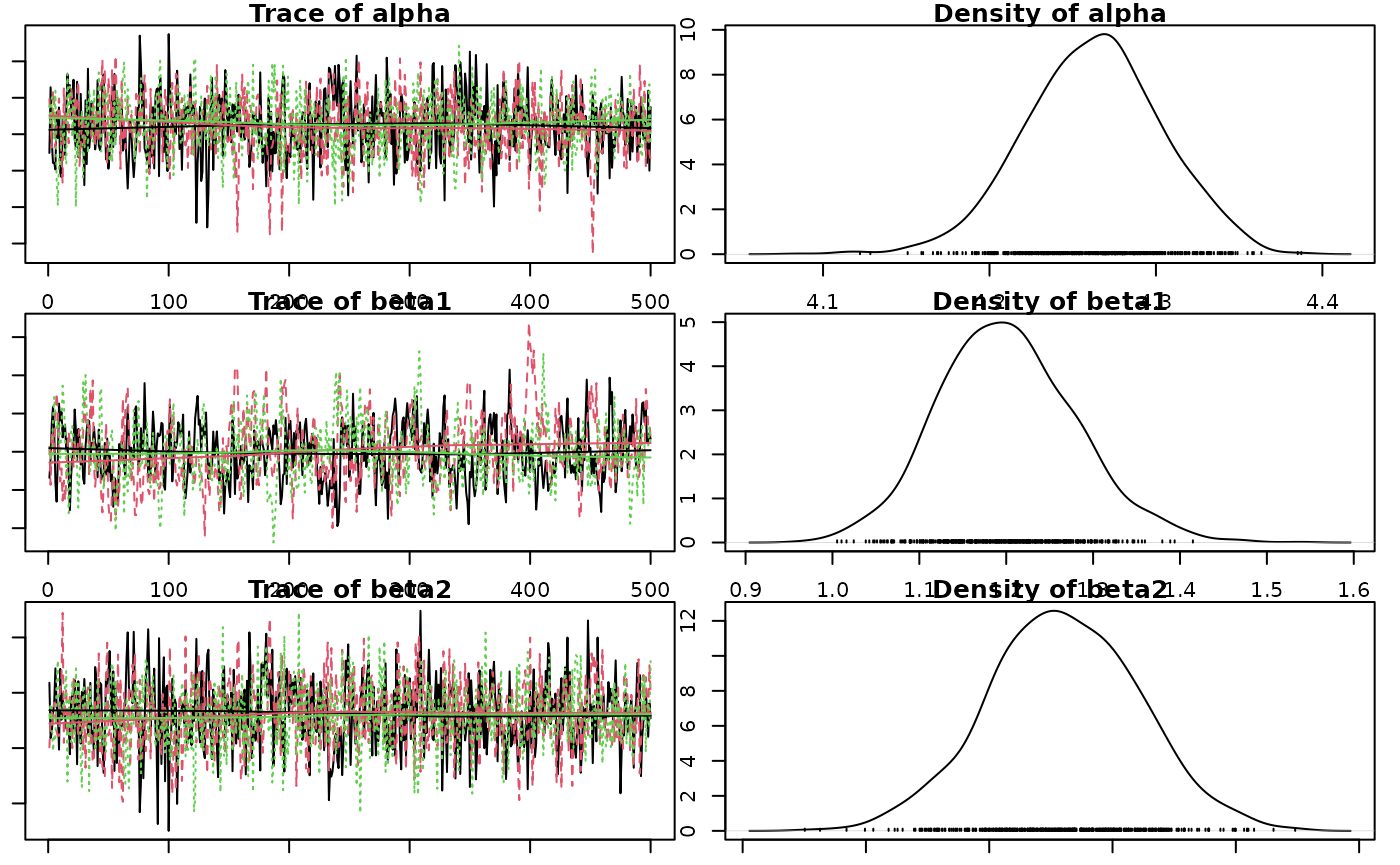
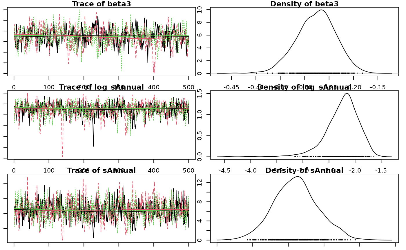
Coefficient Table

Summary table of the posterior probability distribution.

coef(analysis)
#> Warning: The `simplify` argument of `coef()` must be TRUE as of mcmcr 0.4.1.
#> ℹ The deprecated feature was likely used in the base package.
#>   Please report the issue to the authors.
#> This warning is displayed once every 8 hours.
#> Call `lifecycle::last_lifecycle_warnings()` to see where this warning was
#> generated.
#> # A tibble: 6 × 7
#>   term        estimate     sd  zscore   lower   upper   pvalue
#>   <term>         <dbl>  <dbl>   <dbl>   <dbl>   <dbl>    <dbl>
#> 1 alpha         4.26   0.0402 106.     4.18    4.34   0.000666
#> 2 beta1         1.20   0.0713  16.8    1.06    1.34   0.000666
#> 3 beta2        -0.0182 0.0300  -0.627 -0.0758  0.0407 0.507   
#> 4 beta3        -0.275  0.0372  -7.42  -0.349  -0.204  0.000666
#> 5 log_sAnnual  -2.23   0.309   -7.34  -2.99   -1.79   0.000666
#> 6 sAnnual       0.108  0.0300   3.60   0.0501  0.168  0.000666

The estimate is the median by default.

The zscore is mean / sd.

coef(analysis, simplify = TRUE)
#> # A tibble: 6 × 5
#>   term        estimate   lower   upper svalue
#>   <term>         <dbl>   <dbl>   <dbl>  <dbl>
#> 1 alpha         4.26    4.18    4.34   10.6  
#> 2 beta1         1.20    1.06    1.34   10.6  
#> 3 beta2        -0.0182 -0.0758  0.0407  0.980
#> 4 beta3        -0.275  -0.349  -0.204  10.6  
#> 5 log_sAnnual  -2.23   -2.99   -1.79   10.6  
#> 6 sAnnual       0.108   0.0501  0.168  10.6

The s-value is the suprisal value, which is a measure of directionality with respect to zero.

The s-value is zero (unsurprising) when p-value = 1.0 and increases exponentially as p approaches zero.

s = -log_2(p-value) Example: How surprising it would be to throw 10 heads in 10 coin tosses.

A larger s-value provides more evidence against the null hypothesis and support that the data is in the direction of the posterior.

Predictions

Example prediction:

Make predictions by varying Year with other predictors, including the random effect of Annual held constant.

year <- predict(analysis, new_data = "Year")
#> Warning in value[[3L]](cond): beep() could not play the sound due to the following error:
#> Error in play.default(x, rate, ...): no audio drivers are available

library(ggplot2)

ggplot(data = year, aes(x = Year, y = estimate)) +
  geom_point(data = bauw::peregrine, aes(y = Pairs)) +
  geom_line() +
  geom_line(aes(y = lower), linetype = "dotted") +
  geom_line(aes(y = upper), linetype = "dotted") +
  expand_limits(y = 0)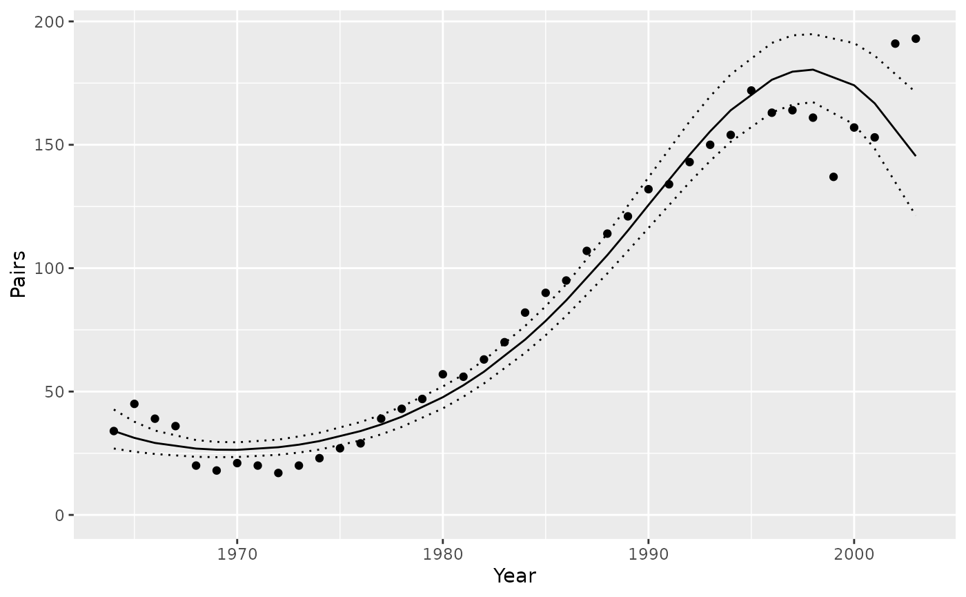

Predict

Predict() queries the model and tells you what the expected number would be for that combination of values specified by new data.

The example below would calculate the annual number of pairs for a typical number of fledged young of 50 (if Eyasses was a parameter in the model).

year <- new_data(data, "Year", ref = list(Eyasses = 50L),
                 obs_only = TRUE) %>%
        predict(analysis, new_data = ., ref_data = ref)

Arguments

new_data: Creates a new data frame to calculate the predictions for.
ref_data: A data frame with 1 row indicating the reference values for calculating the effects size.
- This allows you to calculate the average change relative to something else. In this case ref = list(Eyasses = 50L).

Predict can also take the form:

year <- predict(analysis, new_data = character(0), term = "ePairs")

Where term calls the string of a term in the new expression of the model. By default it is the prediction[i].

New Data

Creates a new data frame to be passed to the predict function.

The idea is that most variables are held constant at a reference level while the variables of interest vary across their range.

year <- new_data(
      data, 
      seq = "Year", 
      ref = list(Eyasses = 50L), 
      obs_only = TRUE) %>%
  predict(analysis, new_data = ., ref_data = ref)

Arguments

seq: The name of columns to vary over. In this example, Year.
- If a factor is named in seq then all levels of the factor are represented.
ref: A named list of reference values for variables not in seq.
- In this case, it is holding the column Eyasses constant at 50L.
obs_only: A list of character vectors indicating the sets of variables to only keep combinations for, i.e. combinations that were observed in the data.
- If obs_only = TRUE then obs_only is set to be seq.
length_out: A count indicating the length of numeric/integer sequences.
- If a factor is named in seq then all levels of the factor are represented (length_out is ignored).
- The exception to this is if the factor is named in obs_only, then only observed factor levels are represented in sequences.