Using odds scaling to accomodate bounded SSDs via ssdtools

Introduction

Currently ssdtools and the associated shiny only includes distributions that are positive (do not include 0) but can exceed 1. This is appropriate for most concentration data that are typically used to derive GVs. However, in the case of direct toxicity assessment of effluents with low toxicity which are inherently bounded between 0 and 1 (depending on whether they represent 0% or 100% sample) a different approach is required, using appropriately bounded statistical distribution(s) for the SSD.

We hypothesize that while the impact of using SSDs unbounded to the right may be small for effluents with a high level of toxicity, this will be very high for effluents with low toxicity.

While it may be possible to add candidate bounded distribution(s) to (shiny)ssdtools, such as the widely used Beta() distribution, this would involve substantial coding effort.

An alternative would be to implement an appropriate transformation of the existing default distribution set to accommodate bounded data. One such appropriate transformation would be to use odds scaling. Transformation to the odds scale can be achieved using the following function:

  odds
#> function (x) 
#> {
#>     x/(1 - x)
#> }

With back-transformation achieved via the corresponding inverse function:

  inv_odds
#> function (x) 
#> {
#>     x/(x + 1)
#> }

Here we compare undertaking an SSD based risk assessment using the toxicity data on their original scale, and ignoring the potential issue that these cannot theoretically take values of greater than 1, whilst all the distributions currently in ssdtools assume the true underlying maximum is Inf.

Methods

The R code that performs the analysis is as follows.

First, we test that our transformation and inversion functions work as expected:

x <- c(0.01, 0.2, 0.5, 0.8)
testthat::expect_identical(x, inv_odds(odds(x)))

Next, we explore some case studies based on toxicity assessments of an effluent sample over time, expressed as a proportion of the tested sample.

Caste study 1

These data are based on a real world discharge example, however they are confidential, so we cannot share the context under which they were collected. However, for this particular case the values were all very low - in some cases much less than 1 percent sample (<0.01 when expressed as a proportion). As they are, these data can be used to asses the impact of accounting for bounding in the SSD in the case where input toxicity data are from the very left hand tail of their theoretical distribution and are therefore highly toxic.

Three highly toxic example datasets of no-significant-effect-concentration toxicity estimates for eleven species, across three different effluent samples. Data are a proportion of the sample.
Spp	sp 1	sp 2	sp 3	sp 4	sp 5	sp 6	sp 7	sp 8	sp 9	sp 10	sp 11
A	0.00490	0.00450	0.00064	0.00330	0.00140	0.00051	0.00062	0.00260	0.00039	0.00520	0.01100
B	0.05500	0.04500	0.01100	0.01700	0.00940	0.00041	0.01500	0.00840	0.01500	0.05000	0.25000
C	0.02600	0.03000	0.01300	0.15000	0.06200	0.00035	0.00980	0.02200	0.11000	0.15000	0.07900

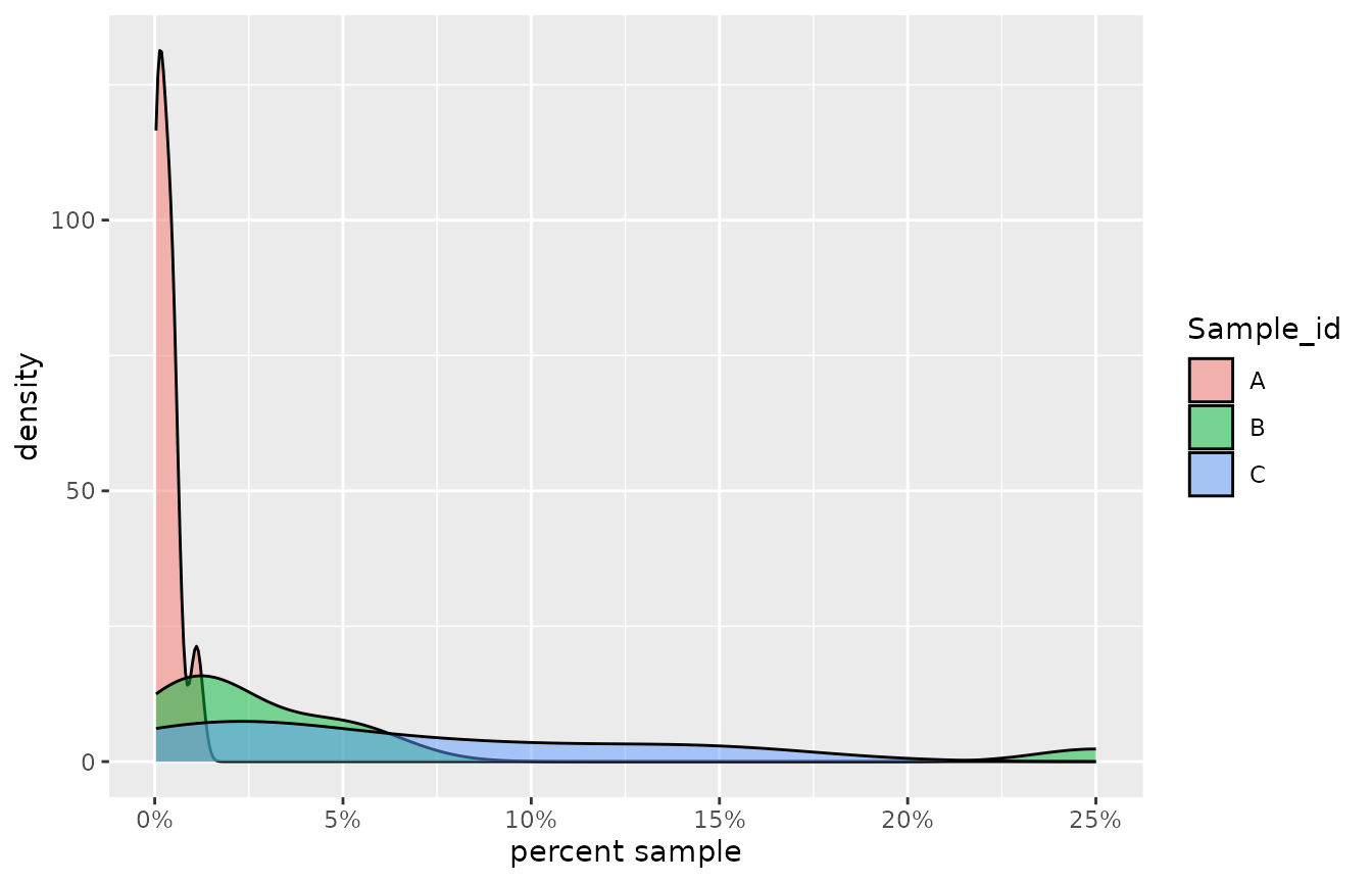
Density plots of the raw toxicity data for three highly toxic effluent samples.

Case study 2

Toxicity estimates from effluent samples may also be on the upper tail of the possible theoretical values of between 0 and 100%. Real world examples might include testing of brine effluent, where some species are relatively insensitive to the elevated salinity and may return toxicity estimates at, or near 100%. To mimic such a scenario, here we simply take the complement to the lower tail toxicity data presented previously, by simply subtracting these observed probabilities from one.

Three low toxicity example datasets of no-significant-effect-concentration toxicity estimates for eleven species, across three different effluent samples. Data are a proportion of the sample.
Spp	sp 1	sp 2	sp 3	sp 4	sp 5	sp 6	sp 7	sp 8	sp 9	sp 10	sp 11
A	1.00	1.00	1.00	1.00	1.00	1.00	1.00	1.00	1.00	0.99	0.99
B	0.95	0.96	0.99	0.98	0.99	1.00	0.98	0.99	0.98	0.95	0.75
C	0.97	0.97	0.99	0.85	0.94	1.00	0.99	0.98	0.89	0.85	0.92

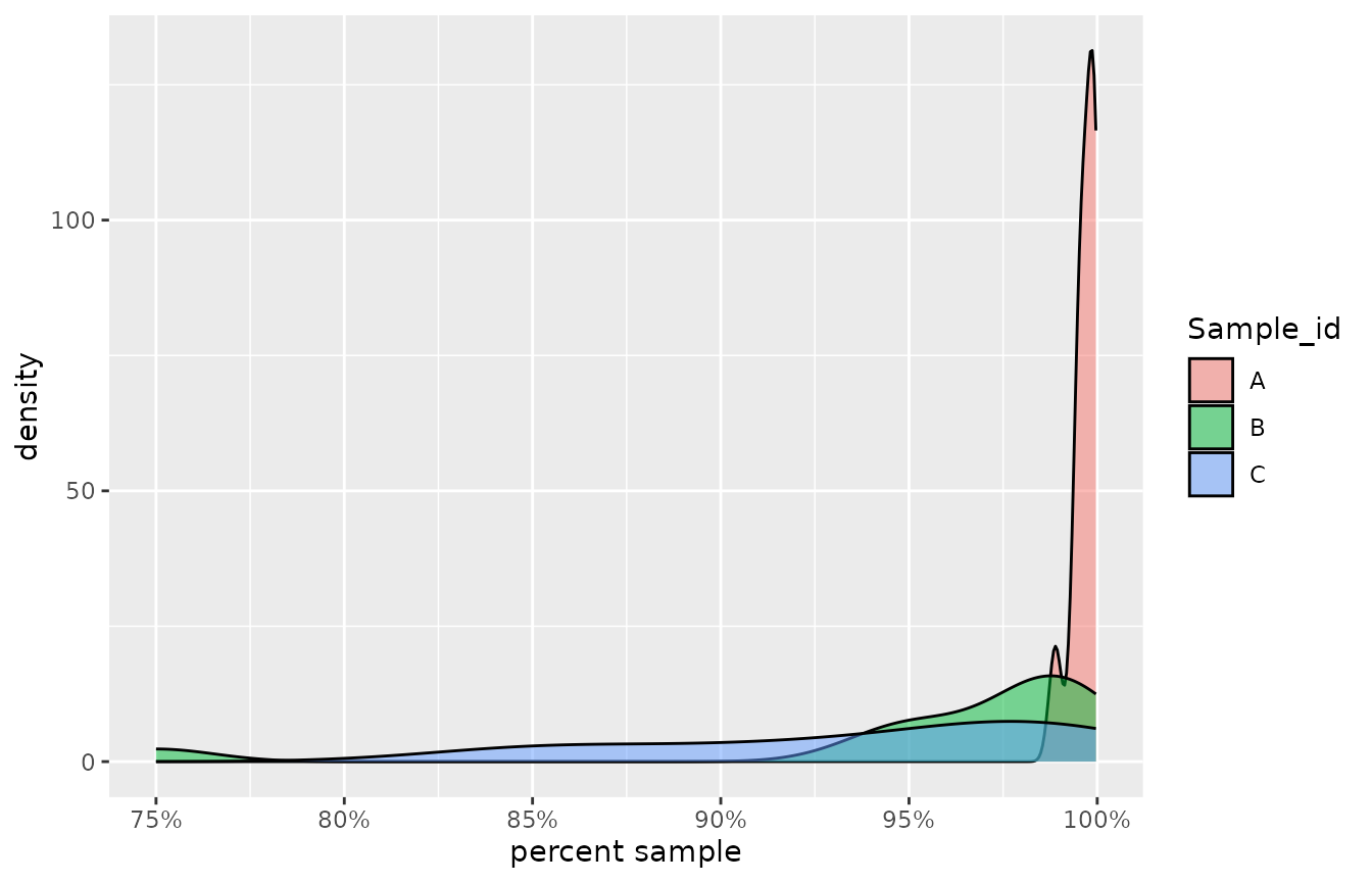
Density plots of the raw toxicity data for three low toxic effluent samples.

We used these three sets of low toxicity and high toxicity examples to examine how the estimated number of dilutions required to reach the different species protection values changed if we model these data on the odds scale to account for the fact that the samples come from a theoretically bounded distribution, compared to if we used the original as though they are from unbounded distributions.

We fitted SSDs to both the original and odds transformed data, using the function ssd_fit_bcanz() from the ssdtools package in R, following the methods outlined in the updated Australian and New Zealand Guidelines for Marine and Freshwater Quality. The only change we made from the recommended defaults settings was to exclude the lognormal-lognormal mixture distribution, as this bi-modal distribution failed to fit to some of our example data.

We obtained 80, 90, 95 and 99 species protection values (0.01, 0.05, 0.1 and 0.2 probability quantiles) from the fitted SSDs for both the odds transformed and original fits. Based on the resulting estimated percentages of the effluent sample, we calculated the number of dilutions required to achieve each protection target.

Findings

We found that there was a substantial difference in the number of dilutions required to meet the desired protection level for the 99 and 95% species protection targets, depending on if the data were modeled on their original scaling which assumes they are unbounded, compared to using the odds scaling.

For both high and low toxicity data examples, performing the SSD modelling on the odds scaling resulted in a higher number of required dilutions compared to when the data are assumed to come from an unbounded distribution.

Number of required dilutions required
Sample_id	proportion	toxicity	original	odds
A	0.01	high toxicity	12400.334615	12462.907418
A	0.05	high toxicity	3602.662073	3608.552642
A	0.10	high toxicity	2240.143162	2242.273474
A	0.20	high toxicity	1323.234195	1323.714740
B	0.01	high toxicity	5581.959795	5955.621547
B	0.05	high toxicity	883.280182	913.213828
B	0.10	high toxicity	415.402067	428.420784
B	0.20	high toxicity	186.197147	190.647411
C	0.01	high toxicity	3185.693513	3743.515970
C	0.05	high toxicity	508.724333	544.892565
C	0.10	high toxicity	227.998540	235.803906
C	0.20	high toxicity	98.370982	98.440106
A	0.01	low toxicity	1.011012	1.044030
A	0.05	low toxicity	1.008014	1.012973
A	0.10	low toxicity	1.006644	1.008188
A	0.20	low toxicity	1.005150	1.004913
B	0.01	low toxicity	1.186611	1.835735
B	0.05	low toxicity	1.125466	1.229141
B	0.10	low toxicity	1.099455	1.131518
B	0.20	low toxicity	1.072930	1.068471
C	0.01	low toxicity	1.234257	1.679255
C	0.05	low toxicity	1.169067	1.261149
C	0.10	low toxicity	1.140361	1.177828
C	0.20	low toxicity	1.108683	1.110628

Expressed as a proportion, the bias in the number of additional required dilutions tended to be higher for the low toxicity data (at the upper extreme of the distribution), compared to the low toxicity data. This would be expected given that these are the toxicity data that are nearest to the upper bound of the distribution. However, because these represent extremely low toxicity examples, the realised number of required dilutions remains very low. For example, based on assuming no bounding, 1.2 dilutions would be required to meet the 99% protection target for the low toxicity example represented by Sample B, compared to 1.8 dilutions when modeled on the odds scale.

While the proportions of required additional dilutions are lower for the high toxicity scenarios relative to the low toxicity scenarios, the actual number of additional dilutions required can be very large. For example, 3,186 dilutions would be required to meet the 99% protection target for the high toxicity example for Sample C. In contrast 3,743 dilutions would be required when modeled on the odds scale.

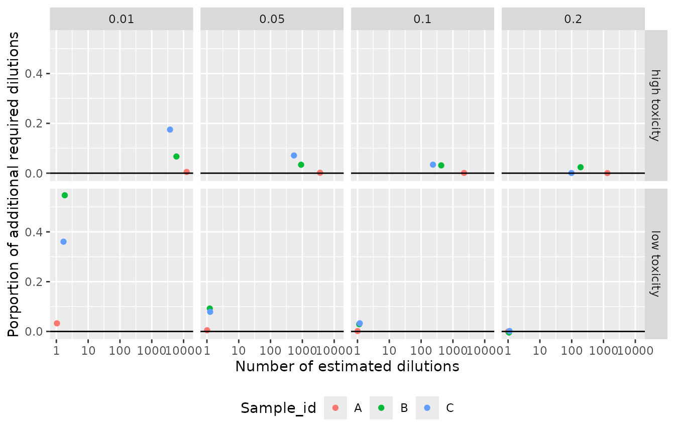
Proportion of additional required dilutions based on SSDs fitted using the original data, when compared to SSDs fitted via odds scaling.

Conclusions and Recommendations

Accommodating bounding of the SSD using odds scaling changes the required number of dilutions to meet species protection targets, particularly when targeting relatively high protection values (e.g. 95 and 99% species protection). In particular, it appears that the target number of dilutions required to meet the protection values are underestimated when bounding is ignored, suggesting that current practice of ignoring the fact that toxicity values come from a bounded distribution in the case of whole effluent toxicity assessment may be resulting in the use of guideline values that do not meet the stated protection targets.

Session Info

The results were generated with the following packages.

#> ─ Session info ───────────────────────────────────────────────────────────────
#>  setting  value
#>  version  R version 4.5.0 (2025-04-11)
#>  os       Ubuntu 24.04.2 LTS
#>  system   x86_64, linux-gnu
#>  ui       X11
#>  language en-US
#>  collate  C.UTF-8
#>  ctype    C.UTF-8
#>  tz       UTC
#>  date     2025-06-13
#>  pandoc   3.1.11 @ /opt/hostedtoolcache/pandoc/3.1.11/x64/ (via rmarkdown)
#>  quarto   NA
#> 
#> ─ Packages ───────────────────────────────────────────────────────────────────
#>  package      * version    date (UTC) lib source
#>  abind          1.4-8      2024-09-12 [1] RSPM
#>  brio           1.1.5      2024-04-24 [1] RSPM
#>  bslib          0.9.0      2025-01-30 [1] RSPM
#>  cachem         1.1.0      2024-05-16 [1] RSPM
#>  chk            0.10.0     2025-01-24 [1] RSPM
#>  cli            3.6.5      2025-04-23 [1] RSPM
#>  codetools      0.2-20     2024-03-31 [3] CRAN (R 4.5.0)
#>  desc           1.4.3      2023-12-10 [1] RSPM
#>  digest         0.6.37     2024-08-19 [1] RSPM
#>  dplyr          1.1.4      2023-11-17 [1] RSPM
#>  evaluate       1.0.3      2025-01-10 [1] RSPM
#>  farver         2.1.2      2024-05-13 [1] RSPM
#>  fastmap        1.2.0      2024-05-15 [1] RSPM
#>  fs             1.6.6      2025-04-12 [1] RSPM
#>  furrr          0.3.1      2022-08-15 [1] RSPM
#>  future         1.58.0     2025-06-05 [1] RSPM
#>  generics       0.1.4      2025-05-09 [1] RSPM
#>  ggplot2      * 3.5.2      2025-04-09 [1] RSPM
#>  globals        0.18.0     2025-05-08 [1] RSPM
#>  glue           1.8.0      2024-09-30 [1] RSPM
#>  goftest        1.2-3      2021-10-07 [1] RSPM
#>  gtable         0.3.6      2024-10-25 [1] RSPM
#>  htmltools      0.5.8.1    2024-04-04 [1] RSPM
#>  jquerylib      0.1.4      2021-04-26 [1] RSPM
#>  jsonlite       2.0.0      2025-03-27 [1] RSPM
#>  knitr          1.50       2025-03-16 [1] RSPM
#>  labeling       0.4.3      2023-08-29 [1] RSPM
#>  lattice        0.22-6     2024-03-20 [3] CRAN (R 4.5.0)
#>  lifecycle      1.0.4      2023-11-07 [1] RSPM
#>  listenv        0.9.1      2024-01-29 [1] RSPM
#>  magrittr       2.0.3      2022-03-30 [1] RSPM
#>  Matrix         1.7-3      2025-03-11 [3] CRAN (R 4.5.0)
#>  parallelly     1.45.0     2025-06-02 [1] RSPM
#>  pillar         1.10.2     2025-04-05 [1] RSPM
#>  pkgconfig      2.0.3      2019-09-22 [1] RSPM
#>  pkgdown        2.1.3      2025-05-25 [1] any (@2.1.3)
#>  pkgload        1.4.0      2024-06-28 [1] RSPM
#>  plyr           1.8.9      2023-10-02 [1] RSPM
#>  purrr          1.0.4      2025-02-05 [1] RSPM
#>  R6             2.6.1      2025-02-15 [1] RSPM
#>  ragg           1.4.0      2025-04-10 [1] RSPM
#>  rbibutils      2.3        2024-10-04 [1] RSPM
#>  RColorBrewer   1.1-3      2022-04-03 [1] RSPM
#>  Rcpp           1.0.14     2025-01-12 [1] RSPM
#>  Rdpack         2.6.4      2025-04-09 [1] RSPM
#>  rlang          1.1.6      2025-04-11 [1] RSPM
#>  rmarkdown      2.29       2024-11-04 [1] RSPM
#>  rprojroot      2.0.4      2023-11-05 [1] RSPM
#>  sass           0.4.10     2025-04-11 [1] RSPM
#>  scales         1.4.0      2025-04-24 [1] RSPM
#>  sessioninfo    1.2.3      2025-02-05 [1] RSPM
#>  ssddata        1.0.0      2021-11-05 [1] RSPM
#>  ssdtools     * 2.3.0.9004 2025-06-13 [1] Github (poissonconsulting/ssdtools@17874d3)
#>  stringi        1.8.7      2025-03-27 [1] RSPM
#>  stringr        1.5.1      2023-11-14 [1] RSPM
#>  systemfonts    1.2.3      2025-04-30 [1] RSPM
#>  testthat       3.2.3      2025-01-13 [1] RSPM
#>  textshaping    1.0.1      2025-05-01 [1] RSPM
#>  tibble         3.3.0      2025-06-08 [1] RSPM
#>  tidyr          1.3.1      2024-01-24 [1] RSPM
#>  tidyselect     1.2.1      2024-03-11 [1] RSPM
#>  TMB            1.9.17     2025-03-10 [1] RSPM
#>  universals     0.0.5      2022-09-22 [1] RSPM
#>  vctrs          0.6.5      2023-12-01 [1] RSPM
#>  waldo          0.6.1      2024-11-07 [1] RSPM
#>  withr          3.0.2      2024-10-28 [1] RSPM
#>  xfun           0.52       2025-04-02 [1] RSPM
#>  yaml           2.3.10     2024-07-26 [1] RSPM
#> 
#>  [1] /home/runner/work/_temp/Library
#>  [2] /opt/R/4.5.0/lib/R/site-library
#>  [3] /opt/R/4.5.0/lib/R/library
#>  * ── Packages attached to the search path.
#> 
#> ──────────────────────────────────────────────────────────────────────────────

Joe Thorley, Rebecca Fisher and David Fox