Introduction
ssdtools is an R package to fit Species Sensitivity
Distributions (SSDs) using Maximum Likelihood and model averaging.
SSDs are cumulative probability distributions that are used to estimate the percent of species that are affected and/or protected by a given concentration of a chemical. The concentration that affects 5% of the species is referred to as the 5% Hazard Concentration (HC5). This is equivalent to a 95% protection value (PC95). For more information on SSDs the reader is referred to Posthuma, Suter II, and Traas (2001).
ssdtools can handle left, right and interval censored
data with two limitations. It is currently only possible to model
average when the distributions have the same number of parameters and
confidence intervals can only be estimated using non-parametric (as
opposed to parametric) bootstrapping.
In order to use ssdtools you need to install R (see
below) or use the Shiny app. The shiny app
includes a user guide. This vignette is a user manual for the R
package.
Philosophy
ssdtools provides the key functionality required to fit
SSDs using Maximum Likelihood and model
averaging in R. It is intended to be used in conjunction with tidyverse packages such as
readr to input data, tidyr and
dplyr to group and manipulate data and ggplot2
(Wickham 2016) to plot data. As such it
endeavors to fulfill the tidyverse manifesto.
Installing
In order to install R (R Core Team 2024) the appropriate binary for the users operating system should be downloaded from CRAN and then installed.
Once R is installed, the ssdtools package can be
installed (together with the tidyverse) by executing the following code
at the R console
install.packages(c("ssdtools", "tidyverse"))The ssdtools package (and ggplot2 package) can then be
loaded into the current session using
Getting Help
To get additional information on a particular function just type
? followed by the name of the function at the R console.
For example ?ssd_gof brings up the R documentation for the
ssdtools goodness of fit function.
For more information on using R the reader is referred to R for Data Science (Wickham and Grolemund 2016).
If you discover a bug in ssdtools please file an issue
with a reprex
(repeatable example) at https://github.com/bcgov/ssdtools/issues.
Inputting Data
Once the ssdtools package has been loaded the next task
is to input some data. An easy way to do this is to save the
concentration data for a single chemical as a column called
Conc in a comma separated file (.csv). Each
row should be the sensitivity concentration for a separate species. If
species and/or group information is available then this can be saved as
Species and Group columns. The
.csv file can then be read into R using the following
data <- read_csv(file = "path/to/file.csv")For the purposes of this manual we use the CCME dataset for boron
from the ssddata
package.
ssddata::ccme_boron
#> # A tibble: 28 × 5
#>    Chemical Species                  Conc Group        Units
#>    <chr>    <chr>                   <dbl> <fct>        <chr>
#>  1 Boron    Oncorhynchus mykiss       2.1 Fish         mg/L
#>  2 Boron    Ictalurus punctatus       2.4 Fish         mg/L
#>  3 Boron    Micropterus salmoides     4.1 Fish         mg/L
#>  4 Boron    Brachydanio rerio        10   Fish         mg/L
#>  5 Boron    Carassius auratus        15.6 Fish         mg/L
#>  6 Boron    Pimephales promelas      18.3 Fish         mg/L
#>  7 Boron    Daphnia magna             6   Invertebrate mg/L
#>  8 Boron    Opercularia bimarginata  10   Invertebrate mg/L
#>  9 Boron    Ceriodaphnia dubia       13.4 Invertebrate mg/L
#> 10 Boron    Entosiphon sulcatum      15   Invertebrate mg/L
#> # ℹ 18 more rows
Fitting Distributions
The function ssd_fit_dists() inputs a data frame and
fits one or more distributions. The user can specify a subset of the
following 9 distributions. Please see the distributions
and model
averaging vignettes for more information regarding appropriate use
of distributions and the use of model-averaged SSDs.
ssd_dists_all()
#> [1] "burrIII3"      "gamma"         "gompertz"      "lgumbel"
#> [5] "llogis"        "llogis_llogis" "lnorm"         "lnorm_lnorm"
#> [9] "weibull"
using the dists argument.
fits <- ssd_fit_dists(ssddata::ccme_boron, dists = c("llogis", "lnorm", "gamma"))Coefficients
The estimates for the various terms can be extracted using the
tidyverse generic tidy function (or the base R generic
coef function).
tidy(fits)
#> # A tibble: 6 × 4
#>   dist   term           est    se
#>   <chr>  <chr>        <dbl> <dbl>
#> 1 llogis locationlog  2.63  0.248
#> 2 llogis scalelog     0.740 0.114
#> 3 lnorm  meanlog      2.56  0.235
#> 4 lnorm  sdlog        1.24  0.166
#> 5 gamma  scale       25.1   7.64
#> 6 gamma  shape        0.950 0.223
Plots
It is generally more informative to plot the fits using the
autoplot generic function (a wrapper on
ssd_plot_cdf()). As autoplot returns a
ggplot object it can be modified prior to plotting. For
more information see the customising
plots vignette.
theme_set(theme_bw()) # set plot theme

autoplot(fits) +
  ggtitle("Species Sensitivity Distributions for Boron") +
  scale_colour_ssd()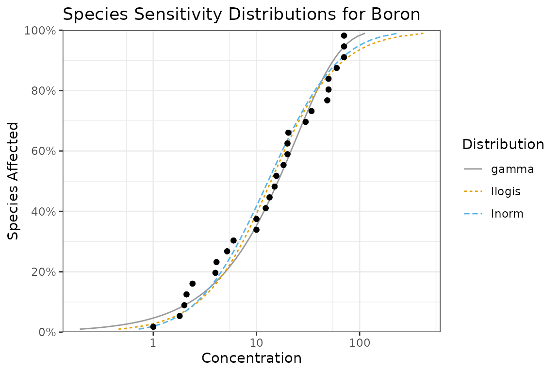
Selecting One Distribution
Given multiple distributions the user is faced with choosing the “best” distribution (or as discussed below averaging the results weighted by the fit).
ssd_gof(fits)
#> Warning: ssd_gof(wt = FALSE) was deprecated in ssdtools 2.3.1.
#> ℹ Please use ssd_gof(wt = TRUE) instead.
#> ℹ Please set the `wt` argument to `ssd_gof()` to be TRUE which will rename the
#>   'weight' column to 'wt' and then update your downstream code accordingly.
#> This warning is displayed once per session.
#> Call `lifecycle::last_lifecycle_warnings()` to see where this warning was
#> generated.
#> # A tibble: 3 × 14
#>   dist   npars  nobs log_lik   aic  aicc delta weight   bic    ad     ks    cvm
#>   <chr>  <int> <int>   <dbl> <dbl> <dbl> <dbl>  <dbl> <dbl> <dbl>  <dbl>  <dbl>
#> 1 llogis     2    28   -119.  241.  241.  3.38  0.11   244. 0.487 0.0994 0.0595
#> 2 lnorm      2    28   -118.  239.  240.  1.40  0.296  242. 0.507 0.107  0.0703
#> 3 gamma      2    28   -117.  238.  238.  0     0.595  240. 0.440 0.117  0.0554
#> # ℹ 2 more variables: at_bound <lgl>, computable <lgl>
The ssd_gof() function returns three test statistics
that can be used to evaluate the fit of the various distributions to the
data.
-
Anderson-Darling
(
ad) statistic, -
Kolmogorov-Smirnov
(
ks) statistic and -
Cramer-von
Mises (
cvm) statistic
and three information criteria
- Akaike’s Information Criterion (
AIC), - Akaike’s Information Criterion corrected for sample size
(
AICc) and - Bayesian Information Criterion (
BIC)
Note if ssd_gof() is called with
pvalue = TRUE then the p-values rather than the statistics
are returned for the ad, ks and cvm tests.
Following Burnham and Anderson (2002)
we recommend the AICc for model selection. The best
predictive model is that with the lowest AICc (indicated by
the model with a delta value of 0 in the goodness of fit
table). In the current example the best predictive model is the gamma
distribution but both the lnorm and llogis distributions have some
support.
For further information on the advantages of an information theoretic approach in the context of selecting SSDs the reader is referred to Fox et al. (2021).
Averaging Multiple Distributions
Often other distributions will fit the data almost as well as the
best distribution as evidenced by delta values < 2 (Burnham and Anderson 2002). In general, the
recommended approach is to estimate the average fit based on the
relative weights of the distributions (Burnham
and Anderson 2002). The AICc based weights are
indicated by the weight column in the goodness of fit
table. A detailed introduction to model averaging can be found in the Model
averaging vignette. A discussion on the recommended set of default
distributions can be found in the Distributions
vignette.
Estimating the Fit
The predict function can be used to generate
model-averaged estimates (or if average = FALSE estimates
for each distribution individual) by bootstrapping. Model averaging is
based on AICc unless the data censored is which case
AICc is undefined. In this situation model averaging is
only possible if the distributions have the same number of parameters
(so that AIC can be used to compare the models).
The resultant object is a data frame of the estimated concentration
(est) with standard error (se) and lower
(lcl) and upper (ucl) 95% confidence limits
(CLs) by percent of species affected (percent). The object
includes the number of bootstraps (nboot) data sets
generated as well as the proportion of the data sets that successfully
fitted (pboot).
boron_pred
#> # A tibble: 99 × 15
#>    dist    proportion   est    se    lcl   ucl    wt level est_method ci_method
#>    <chr>        <dbl> <dbl> <dbl>  <dbl> <dbl> <dbl> <dbl> <chr>      <chr>
#>  1 average       0.01 0.267 0.402 0.0419  1.53     1  0.95 multi      weighted_…
#>  2 average       0.02 0.531 0.518 0.110   2.03     1  0.95 multi      weighted_…
#>  3 average       0.03 0.783 0.615 0.198   2.50     1  0.95 multi      weighted_…
#>  4 average       0.04 1.02  0.701 0.300   2.89     1  0.95 multi      weighted_…
#>  5 average       0.05 1.26  0.782 0.407   3.29     1  0.95 multi      weighted_…
#>  6 average       0.06 1.48  0.859 0.520   3.72     1  0.95 multi      weighted_…
#>  7 average       0.07 1.71  0.934 0.645   4.16     1  0.95 multi      weighted_…
#>  8 average       0.08 1.93  1.01  0.769   4.58     1  0.95 multi      weighted_…
#>  9 average       0.09 2.16  1.08  0.896   4.95     1  0.95 multi      weighted_…
#> 10 average       0.1  2.38  1.15  1.03    5.33     1  0.95 multi      weighted_…
#> # ℹ 89 more rows
#> # ℹ 5 more variables: boot_method <chr>, nboot <dbl>, pboot <dbl>,
#> #   dists <list>, samples <list>
The data frame of the estimates can then be plotted together with the
original data using the ssd_plot() function to summarize an
analysis. Once again the returned object is a ggplot object
which can be customized prior to plotting.
ssd_plot(ssddata::ccme_boron, boron_pred,
  color = "Group", label = "Species",
  xlab = "Concentration (mg/L)", ribbon = TRUE
) +
  expand_limits(x = 5000) + # to ensure the species labels fit
  ggtitle("Species Sensitivity for Boron") +
  scale_colour_ssd()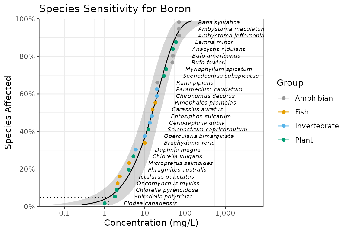
In the above plot the model-averaged 95% confidence interval is indicated by the shaded band and the model-averaged 5%/95% Hazard/Protection Concentration (HC5/ PC95) by the dotted line. Hazard/Protection concentrations are discussed below.
Hazard/Protection Concentrations
The 5% hazard concentration (HC5) is the concentration that affects 5% of the species tested. This is equivalent to the 95% protection concentration which protects 95% of species (PC95). The hazard and protection concentrations are directly interchangeable, and terminology depends simply on user preference.
The hazard/protection concentrations can be obtained using the
ssd_hc() function, which can be used to obtain any desired
percentage value. The fitted SSD can also be used to determine the
percentage of species protected at a given concentration using
ssd_hp().
withr::with_seed(99, {
  boron_hc5 <- ssd_hc(fits, proportion = 0.05, ci = TRUE)
  print(boron_hc5)
  boron_pc <- ssd_hp(fits, conc = boron_hc5$est, ci = TRUE)
  print(boron_pc)
})
#> # A tibble: 1 × 15
#>   dist    proportion   est    se   lcl   ucl    wt level est_method ci_method
#>   <chr>        <dbl> <dbl> <dbl> <dbl> <dbl> <dbl> <dbl> <chr>      <chr>
#> 1 average       0.05  1.32 0.850 0.370  3.67     1  0.95 multi      weighted_sa…
#> # ℹ 5 more variables: boot_method <chr>, nboot <dbl>, pboot <dbl>,
#> #   dists <list>, samples <list>
#> Warning: ssd_hp(proportion = FALSE) was deprecated in ssdtools 2.3.1.
#> ℹ Please use ssd_hp(proportion = TRUE) instead.
#> ℹ Please set the `proportion` argument to `ssd_hp()` to be TRUE which will
#>   cause it to return hazard proportions instead of percentages then update your
#>   downstream code accordingly.
#> This warning is displayed once per session.
#> Call `lifecycle::last_lifecycle_warnings()` to see where this warning was
#> generated.
#> # A tibble: 1 × 15
#>   dist     conc   est    se   lcl   ucl    wt level est_method ci_method
#>   <chr>   <dbl> <dbl> <dbl> <dbl> <dbl> <dbl> <dbl> <chr>      <chr>
#> 1 average  1.32     5  3.23 0.587  12.8     1  0.95 multi      weighted_samples
#> # ℹ 5 more variables: boot_method <chr>, nboot <dbl>, pboot <dbl>,
#> #   dists <list>, samples <list>
Censored Data
Censored data is that for which only a lower and/or upper limit is
known for a particular species. If the right argument in
ssd_fit_dists() is different to the left
argument then the data are considered to be censored.
Let’s produce some left censored data.
boron_censored <- ssddata::ccme_boron |>
  dplyr::mutate(left = Conc, right = Conc)

boron_censored$left[c(3, 6, 8)] <- NA
As the sample size n is undefined for censored data,
AICc cannot be calculated. However, if all the models have
the same number of parameters, the AIC delta
values are identical to those for AICc. For this reason,
ssdtools only permits model averaging of censored data for
distributions with the same number of parameters. We can call only the
default two parameter models using
ssd_dists_bcanz(n = 2).
dists <- ssd_fit_dists(boron_censored,
  dists = ssd_dists_bcanz(n = 2),
  left = "left", right = "right"
)
There are less goodness-of-fit statistics available for fits to
censored data (currently just AIC and
BIC).
ssd_gof(dists)
#> # A tibble: 5 × 14
#>   dist    npars  nobs log_lik   aic  aicc delta weight   bic    ad    ks   cvm
#>   <chr>   <int> <int>   <dbl> <dbl> <dbl> <dbl>  <dbl> <dbl> <dbl> <dbl> <dbl>
#> 1 gamma       2    NA   -109.  222.    NA 0      0.376    NA    NA    NA    NA
#> 2 lgumbel     2    NA   -112.  228.    NA 5.67   0.022    NA    NA    NA    NA
#> 3 llogis      2    NA   -111.  226.    NA 3.70   0.059    NA    NA    NA    NA
#> 4 lnorm       2    NA   -110.  224.    NA 1.52   0.176    NA    NA    NA    NA
#> 5 weibull     2    NA   -109.  222.    NA 0.046  0.367    NA    NA    NA    NA
#> # ℹ 2 more variables: at_bound <lgl>, computable <lgl>
The model-averaged predictions are calculated using
AIC
ssd_hc(dists, average = FALSE)
#> # A tibble: 5 × 15
#> dist proportion est se lcl ucl wt level est_method ci_method
#> <chr> <dbl> <dbl> <dbl> <dbl> <dbl> <dbl> <dbl> <chr> <chr>
#> 1 gamma 0.05 0.674 NA NA NA 0.376 0.95 cdf percentile
#> 2 lgumbel 0.05 1.51 NA NA NA 0.0221 0.95 cdf percentile
#> 3 llogis 0.05 1.15 NA NA NA 0.0590 0.95 cdf percentile
#> 4 lnorm 0.05 1.32 NA NA NA 0.176 0.95 cdf percentile
#> 5 weibull 0.05 0.752 NA NA NA 0.367 0.95 cdf percentile
#> # ℹ 5 more variables: boot_method <chr>, nboot <int>, pboot <dbl>,
#> # dists <list>, samples <list>
ssd_hc(dists)
#> # A tibble: 1 × 15
#> dist proportion est se lcl ucl wt level est_method ci_method
#> <chr> <dbl> <dbl> <dbl> <dbl> <dbl> <dbl> <dbl> <chr> <chr>
#> 1 average 0.05 0.859 NA NA NA 1 0.95 multi weighted_sa…
#> # ℹ 5 more variables: boot_method <chr>, nboot <int>, pboot <dbl>,
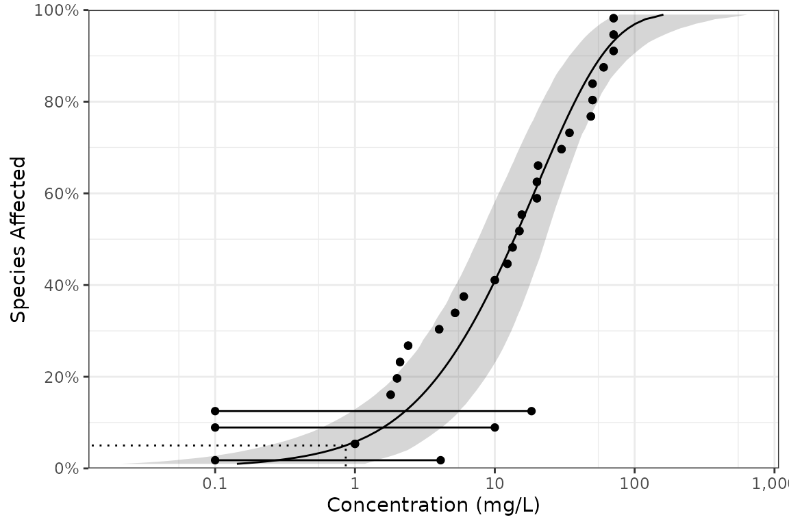
#> # dists <list>, samples <list>The confidence intervals can currently only be generated for censored data using non-parametric bootstrapping. The horizontal lines in the plot indicate the censoring (range of possible values).
withr::with_seed(99, {
  pred <- predict(dists, ci = TRUE, parametric = FALSE)
})

ssd_plot(boron_censored, pred,
  left = "left", right = "right",
  xlab = "Concentration (mg/L)"
)
References
Licensing
Copyright 2015-2023 Province of British Columbia
Copyright 2021 Environment and Climate Change Canada
Copyright 2023-2025 Australian Government Department of Climate Change,
Energy, the Environment and Water
The documentation is released under the CC BY 4.0 License
The code is released under the Apache License 2.0