Boreal Caribou Simulations Analysis

Dalgarno, S., Thorley, J.L., Boulanger, J. & Pearson, A.

Background

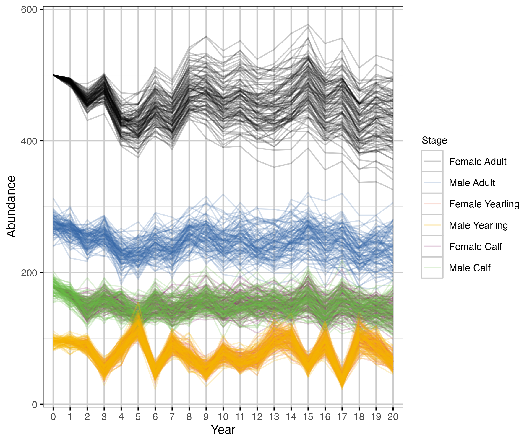
The objectives of this analysis are to:

• Simulate Boreal Caribou recruitment and survival data from key demographic and sampling parameters.
  
• Assess the ability of various statistical methods to recover known parameter values from simulated data.

One hundred recruitment and survival data sets were simulated from a single set of demographic (table 1) and sampling (table 2) parameters for each of 5 coverage scenarios (table 3). Coverage scenarios included variation in the number of collared adult females (for survival data) and the proportion of groups observed in hypothetical composition surveys (for recruitment data). Realistic parameter values for survival/fecundity rates and population simulation were derived from observed values in anonymized example datasets. The simulated population is stable (i.e., lambda close to 1; table 4). See this bbousims vignette for more information on how survival and recruitment data are simulated, given the parameter values in table 1 and table 2.

Statistical methods compared include a Bayesian model with year as fixed effect, a Bayesian model with year as random effect, and a frequentist retro model. See this bboutools vignette for more details on the statistical methods. All Bayesian models had uninformative priors.

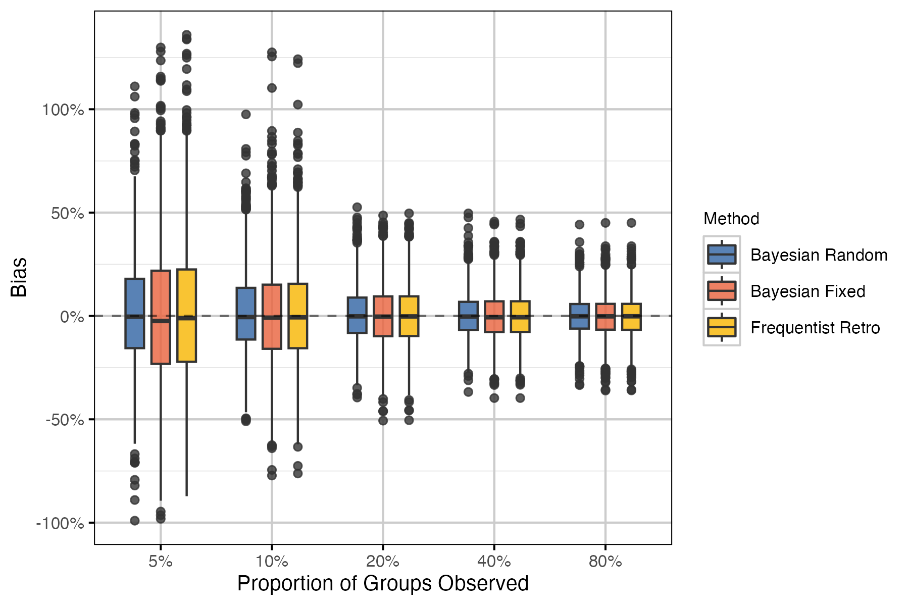
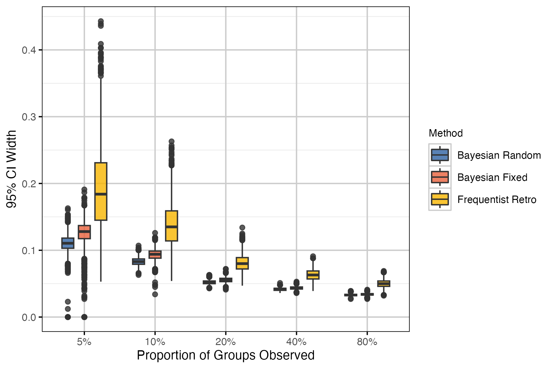
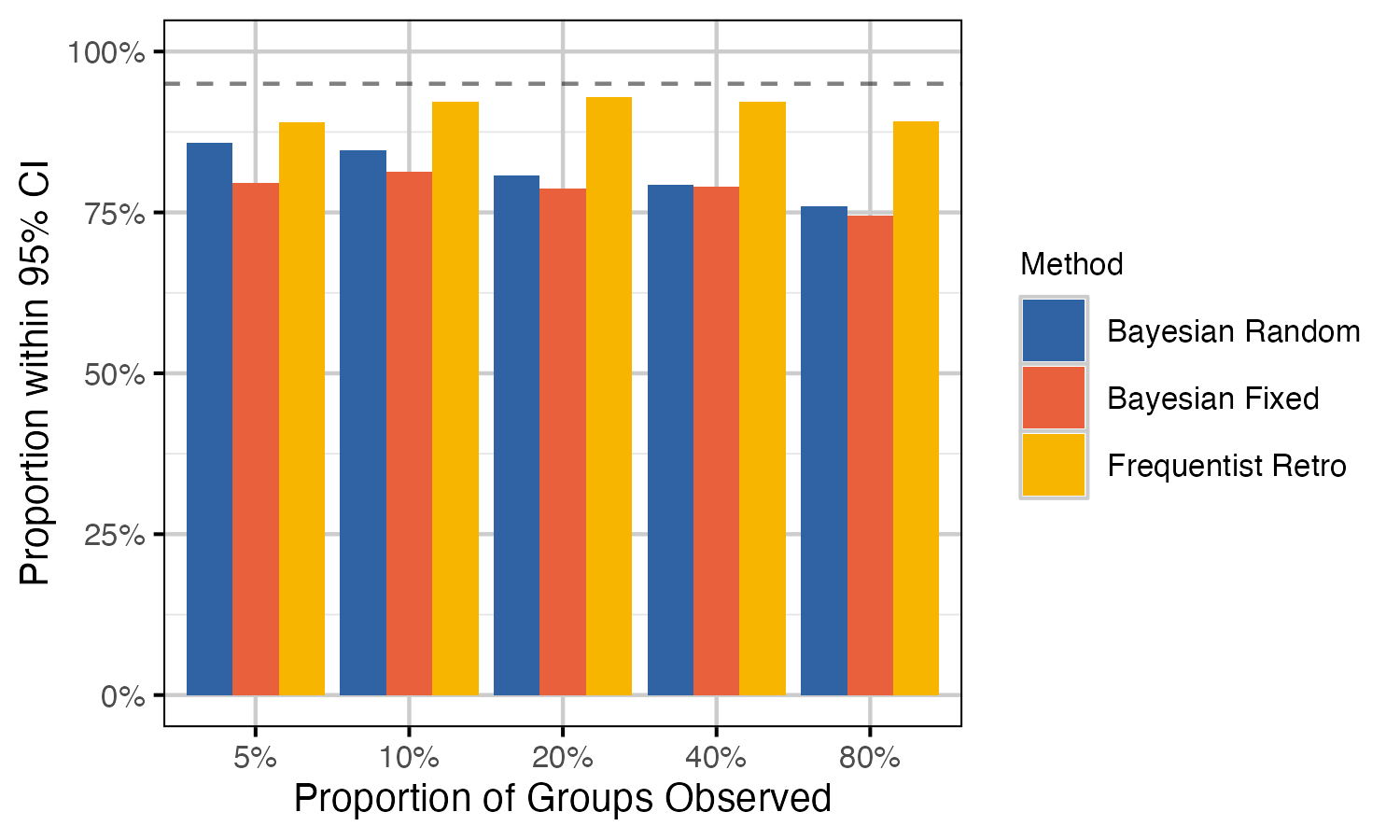
Performance metrics used include bias, precision and coverage. Bias is a measure of the degree to which the estimate over- or under-estimates the true value. An unbiased estimator is one for which the mean bias across all estimates is zero. Precision is simply the difference between the upper and lower limits of the 95% CI. Note that for Bayesian models CI refers to the credible interval, whereas CI represents the confidence interval in frequentist methods. Coverage is the proportion of estimates for which the 95% CI contain the true value. All performance metrics are visualized as boxplots, which display the median and 95% interquartile range. Each boxplot is a summary of 2000 points (i.e., 100 simulations by 20 years).

Frequentist retro methods fail to estimate standard error (and 95% CI) for annual survival when there are 0 observed mortalities. In these cases, the annual population growth (lambda) estimates are also missing 95% CI. It is important to note that the precision plots exclude these values and the coverage plots assume that the known value is not within the 95% CI. The number (and proportion) of these cases is summarized for each coverage scenario in table 5 and 6.

Results

Population

Table 1. Parameter values for generation of survival and fecundity rates.

Parameter	Value
Survival Adult Female Intercept	0.86
Survival Adult Female Annual SD	0.35
Survival Adult Female Month SD	0.10
Survival Adult Female Annual within Month SD	0.01
Survival Adult Female Trend	0.00
Survival Calf Female Intercept	0.50
Survival Calf Female Annual SD	0.35
Survival Calf Female Month SD	0.10
Survival Calf Female Annual within Month SD	0.01
Survival Calf Female Trend	0.00
Calves per Adult Female Intercept	0.70
Calves per Adult Female Intercept Annual SD	0.00
Calves per Adult Female Trend	0.00

Table 2. Parameter values for population simulation.

Parameter	Value
Simulations	100
Years	20
Initial Adult Females	500
Proportion Adult Female	0.65
Proportion Yearling Female	0.5
Month Collared	1
Month Composition Survey	9
Mean Group Size	5
Minimum Group Size	2
Probabiility Unsexed Adult Female	0.01
Probabiility Unsexed Adult Male	0.01
Group Coverage	5%, 10%, 30%, 50%, 80%
Collared Adult Females	5, 10, 20, 30, 50
Probability Uncertain Collar Survival	0
Probability Uncertain Collar Mortality	0.01

Table 3. Scenarios for population simulation.

survival_adult_female	coverage	group_coverage	collared_adult_females
0.86	1	0.05	5
0.86	2	0.10	10
0.86	3	0.30	20
0.86	4	0.50	30
0.86	5	0.80	50

Table 4. Key demographic summary parameters for model Caribou population

Parameter	Value
Lambda	0.9916254
Recruitment	0.1194539
Calf-Cow Ratio	0.2713178
Adult Female Survival	0.8600000
Calf Survival	0.5000000
Calves per Adult Female	0.7000000

Figure 1. Population by stage for 100 simulations.

Survival

Figure 2. Bias (% difference) in annual survival point estimates and known survival for 100 simulations and 20 years, by sample size and statistical method.

Figure 3. Precision (95% CI width) in estimated annual survival for 100 simulations and 20 years, by sample size and statistical method. ‘Frequentist Retro’ estimates with standard error of 0 are included with CI width of 0. See table 5 for the number of estimates with SE of 0 in each coverage scenario.

Figure 4. Proportion of the estimated annual survival 95% CI that contains the known value for 100 simulations and 20 years, by sample size and statistical method. In cases where the ‘Frequentist Retro’ estimated SE is 0, we assumed that the known value is outside the 95% CI.

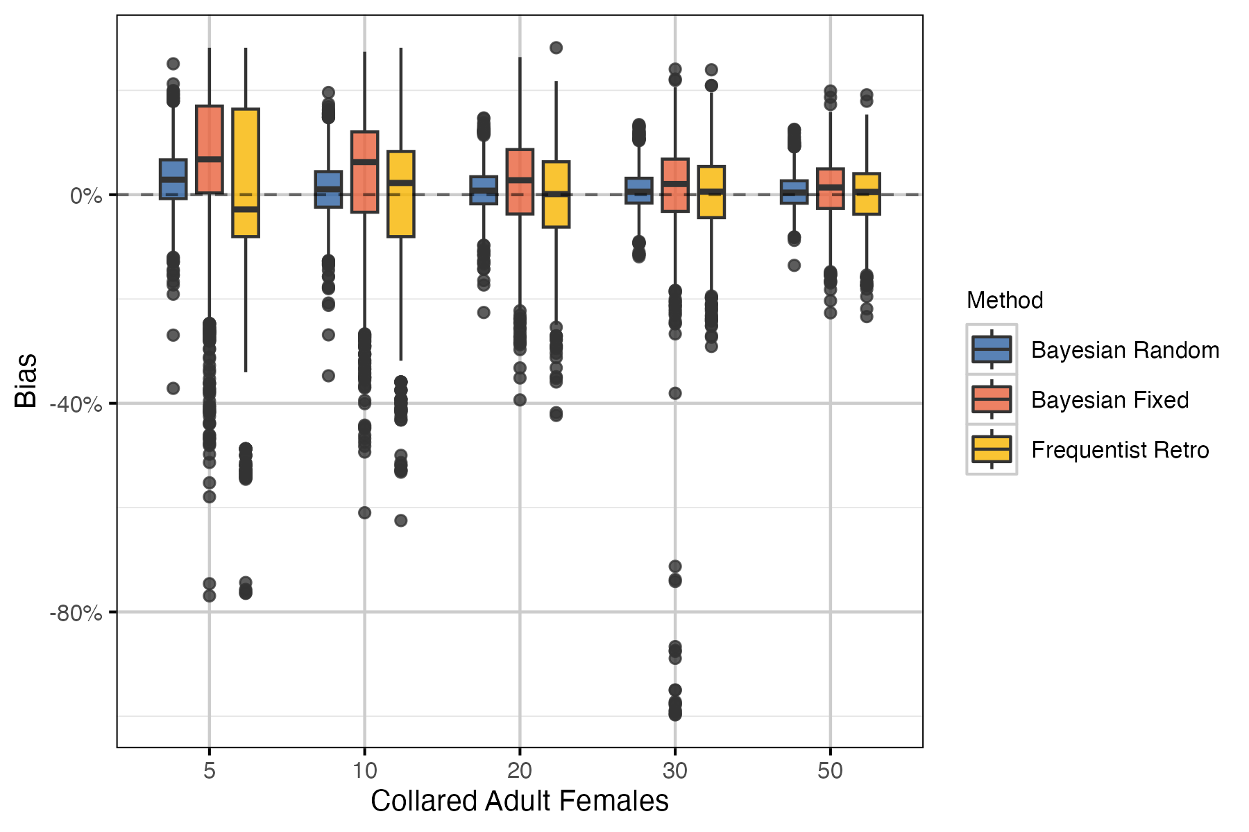
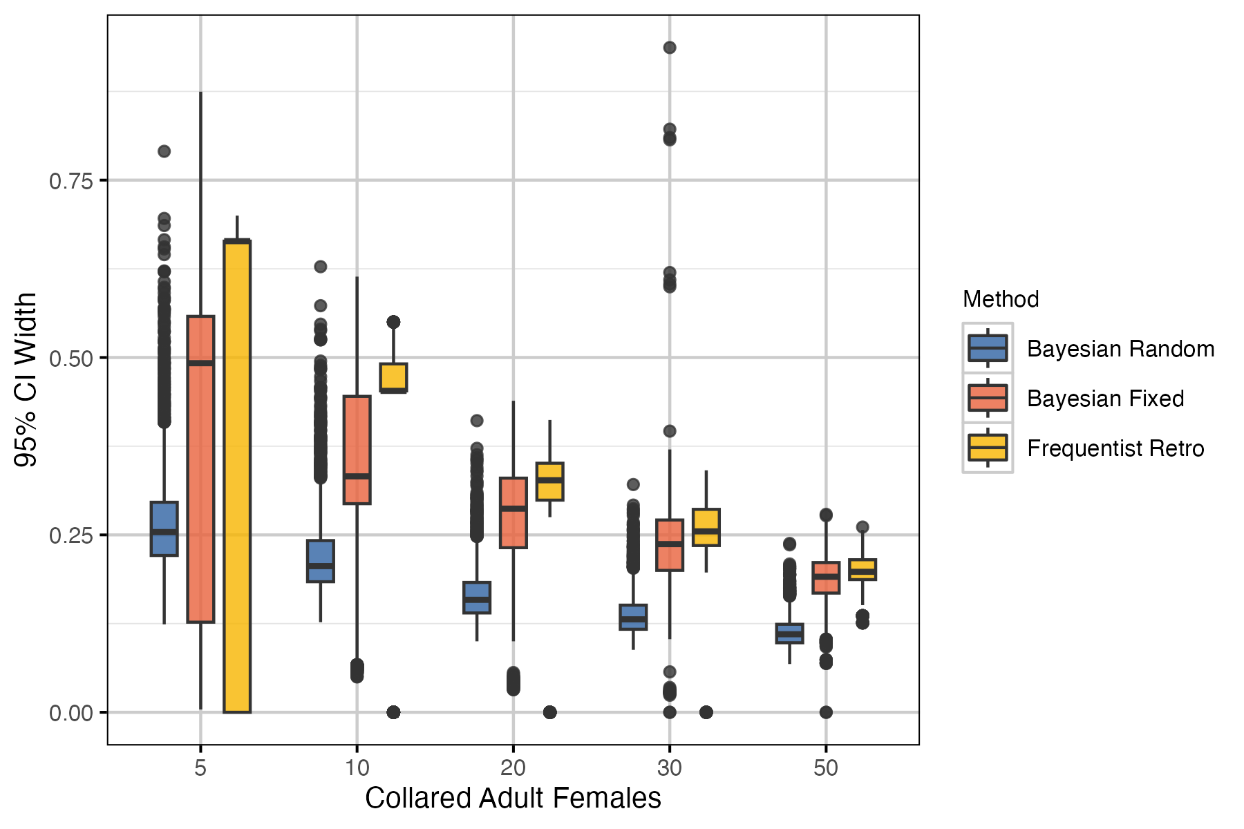
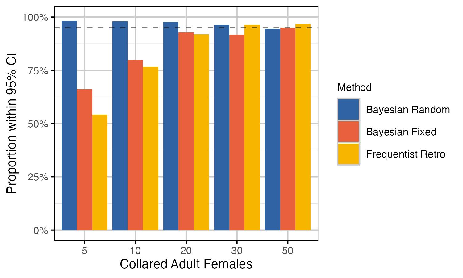
Table 5. Number and proportion (%) of annual survival estimates with no standard error (SE is 0). This occurs with the ‘Frequentist Retro’ methods when there are 0 mortalities.

Collars	No SE	% No SE
5	877	43.85
10	373	18.65
20	85	4.25
30	16	0.80
50	0	0.00

Recruitment

Figure 5. Bias (% difference) in annual recruitment point estimates and known survival for 100 simulations and 20 years, by proportion of groups observed and statistical method.

Figure 6. Precision (95% CI width) in estimated annual recruitment for 100 simulations and 20 years, by proportion of groups observed and statistical method.

Figure 7. Proportion of the estimated annual recruitment 95% CI that contains the known value for 100 simulations and 20 years, by proportion of groups observed and statistical method.

Growth

Figure 8. Bias (% difference) in annual population growth (lambda) point estimates and known survival for 100 simulations and 20 years, by coverage scenario and statistical method.

Figure 9. Precision (95% CI width) in estimated annual population growth (lambda) for 100 simulations and 20 years, by coverage scenario and statistical method. ‘Frequentist Retro’ estimates with missing CI are included with CI width of 0. See table 6 for the number of estimates with missing CI in each coverage scenario.

Figure 10. Proportion of the estimated annual population growth 95% CI that contains the known value for 100 simulations and 20 years, by coverage scenario and statistical method. In cases where the estimate was missing CI, we assumed that the known value is outside the 95% CI. This occurs in the ‘Frequentist Retro’ method when there are 0 mortalities and estimated SE in survival is 0.

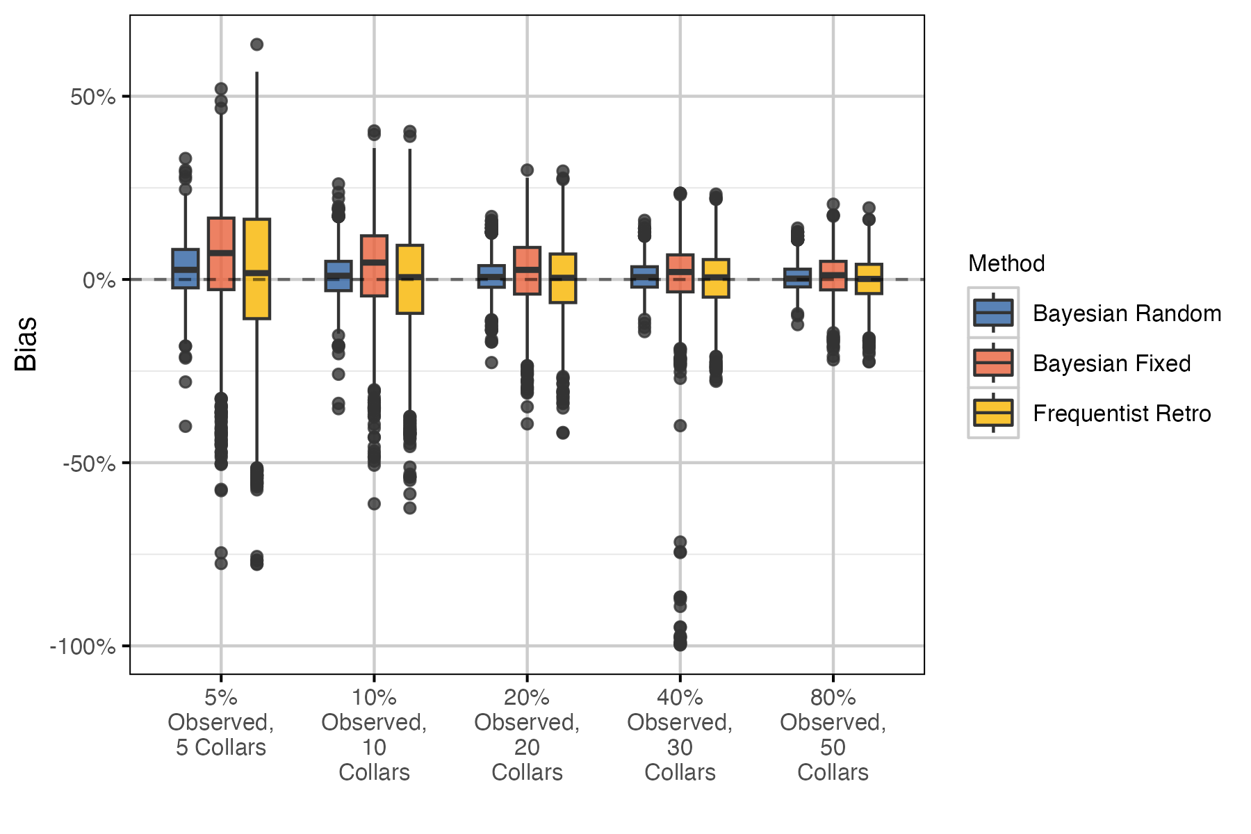
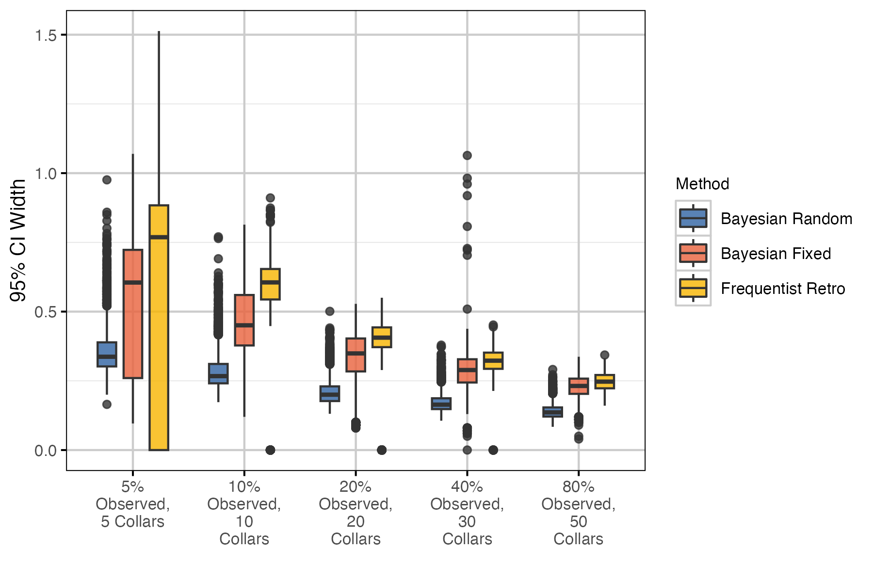
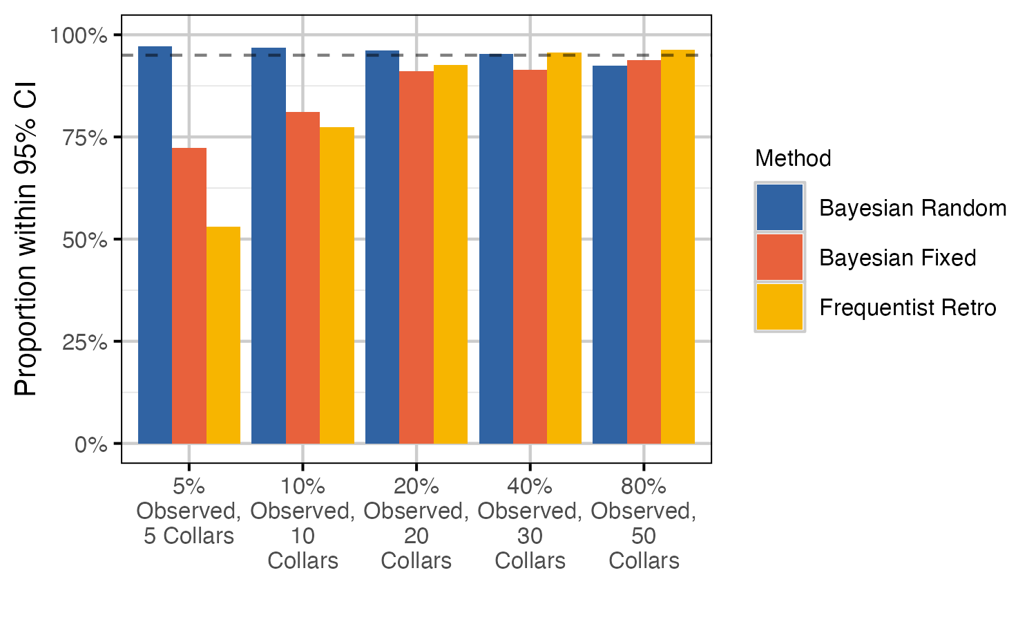
Table 6. Number and proportion (%) of annual population growth (lambda) estimates with no CI due to missing survival SE. This occurs in the ‘Frequentist Retro’ method when there are 0 mortalities.

Coverage	No CI	% No CI
5% Observed, 5 Collars	877	43.85
10% Observed, 10 Collars	373	18.65
20% Observed, 20 Collars	85	4.25
40% Observed, 30 Collars	16	0.80
80% Observed, 50 Collars	0	0.00

Discussion

For the survival model, higher sample size resulted in reduced bias, higher precision and higher coverage for all statistical methods. The Bayesian random effects model performed best, with improvement over other methods particularly at lower sample sizes.

Results for the recruitment model were similar, although the difference between methods was less extreme. In general, the Bayesian random effects model performed best. Surprisingly, coverage was reduced with higher proportion of groups observed in the Bayesian recruitment models. We suspect that this is caused by higher precision leading to a higher tendency for the 95% CI to not include the true value.

The growth predictions are derived from the recruitment and survival estimates and thus, it is unsurprising that the Bayesian random effects model performed best.

A consequence of modeling year as a random effect is that individual estimates are pulled in toward the grand mean, especially when estimates have low precision or are more extreme (Kery and Schaub 2011). This simulation analysis demonstrates that this ‘shrinkage’ is desirable as the random effects model tends to be more skeptical of extreme values. Extreme values are likely to result from the sampling process rather than the ecological processes, especially at low sample sizes.

Kery, Marc, and Michael Schaub. 2011. Bayesian Population Analysis Using WinBUGS : A Hierarchical Perspective. Boston: Academic Press. http://www.vogelwarte.ch/bpa.html.