Analytic Methods for Estimation of Boreal Caribou Survival, Recruitment and Population Growth

Bayesian vs Frequentist Framework

The frequentist (Maximum Likelihood) framework selects the parameter values which if they were true would be most likely to give rise to the data. It assumes that all possible survival and recruitment values are equally likely to be true. The confidence intervals (CIs) are invalid with small sample size.

The Bayesian framework selects parameter values which are most likely to be true given the data. It allows incorporation of biological knowledge. The credible intervals (CIs) represent the actual uncertainty irrespective of the sample size.

Most models can be fit in a Bayesian or frequentist framework.

Fixed vs Random Effects

When a categorical variable is treated as a fixed effect each parameter value is estimated in isolation. In contrast, when it is treated as a random effect the parameter values are assumed to be drawn from a common underlying distribution which allows the typical values to be estimated and each parameter estimate to be influenced by the other ones.

The use of random effects is especially beneficial when some months/years have sparse or missing data. In the case of sparse data or extreme values, estimates will tend to be pulled toward the grand mean, a behaviour known as ‘shrinkage’ (kery_bayesian_2011?). For missing data, the estimate will be equal to the mean. Shrinkage may not be desired if extreme values are likely to represent the true value (e.g., numerous wolf attacks in one year). In this case, a fixed effect model would yield more reliable estimates.

Fixed and random effects can be used in Bayesian or frequentist models.

Maximum Likelihood vs Posterior Probability

The frequentist approach simply identifies the parameter values that maximize the likelihood, i.e., have the greatest probability of having produced the data if they were true. It does this by searching parameter space for the combination of parameter values with the Maximum Likelihood. Parameter estimates for random effects can be estimated using the Laplace approximation (i.e., with software packages TMB or Nimble). The CIs are calculated using the standard errors, assuming that the likelihood is normally distributed. This approach has the advantage of being fast.

The Bayesian approach multiplies the likelihood by the prior probability of the parameter values being true to get the posterior probability of the parameter values being true based on the data. Bayesian methods repeatedly sample from the posterior probability distributions using MCMC (Monte Carlo Markov Chain) methods. This approach has the advantage of allowing derived parameters such as the population growth rate to be easily estimated with full uncertainty from the primary survival and recruitment parameters.

To demonstrate, we use an anonymized data set to compare annual survival estimates from a:

• Bayesian model with fixed year effect.
  
• Bayesian model with random year effect.
  
• Maximum Likelihood model with fixed year effect.
  
• Maximum Likelihood model with random year effect.

Observed data (black points) are shown as the mean monthly survival by year, weighted by the square root of the number of collars. Transparency of the black points shows the mean $\sqrt(n)$.

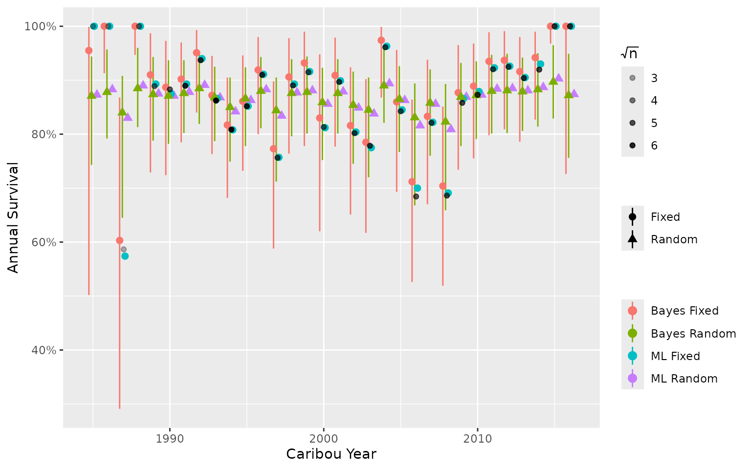
In this example, Maximum Likelihood and Bayesian models of the same type (i.e., fixed or random) have similar estimates because the Bayesian model priors are not informative. Estimates from random effect models tend to be pulled toward the mean. Estimates from the fixed effect models more closely match the observed data, including extreme values. Note, there is no functionality in bboutools to get confidence intervals on predictions (i.e., derived parameters) for Maximum Likelihood models. This is a more straightforward task with Bayesian models.

bboutools

bboutools provides the option to estimate parameter values using a Maximum Likelihood or a fully Bayesian approach. Random effects are used where appropriate by default. The Bayesian approach also uses biologically reasonable, weakly informative priors by default. bboutools provides relatively simple general models that can be used to compare survival, recruitment and population growth estimates across jurisdictions.

By default, the bboutools Bayesian method saves 1,000 MCMC samples from each of three chains (after discarding the first halves). The number of samples saved can be adjusted with the niters argument. With niters set, the user can simply increment the thinning rate as required to achieve convergence. This process is automated in the Shiny app.

Survival Model

The survival model with annual random effect and trend is specified below in a simplified form of the BUGS language for readability. The same model code is used for both the Bayesian and frequentist methods.

b0 ~ Normal(3, 10)
bYear ~ Normal(0, 2)

sMonth ~  Exponential(1)
for(i in 1:nMonth)  bMonth[i] ~ Normal(0, sMonth)

sAnnual ~ Exponential(1)
for(i in 1:nAnnual)  bAnnual[i] ~ Normal(0, sAnnual)

for(i in 1:nObs) {
  logit(eSurvival[i]) = b0 + bMonth[Month[i]] + bAnnual[Annual[i]] + bYear * Year[i]
  Mortalities[i] ~ Binomial(1 - eSurvival[i], StartTotal[i])
}

Recruitment Model

The recruitment model with annual random effect and year trend is specified below in a simplified form of the BUGS language for readability. Group-level observations are aggregated by caribou year prior to model fitting.

b0 ~ Normal(-1, 5)
bYear ~ Normal(0, 1)

adult_female_proportion ~ Beta(65, 35)

sAnnual ~  Exponential(1)
for(i in 1:nAnnual)  bAnnual[i] ~ Normal(0, sAnnual)

for(i in 1:nAnnual) {
  FemaleYearlings[i] ~ Binomial(sex_ratio, Yearlings[i])
  Cows[i] ~ Binomial(adult_female_proportion, CowsBulls[i])
  OtherAdultsFemales[i] ~ Binomial(adult_female_proportion, UnknownAdults[i])
  log(eRecruitment[i]) <- b0 + bAnnual[Annual[i]] + bYear * Year[i]
  AdultsFemales[i] <- max(FemaleYearlings[i] + Cows[i] + OtherAdultsFemales[i], 1)
  Calves[i] ~ Binomial(eRecruitment[i], AdultsFemales[i])
}

In the frequentist approach, demographic stochasticity is removed from the model because it is not possible to estimate discrete latent variables using Laplace approximation. This has a minimal effect on estimates. The adjusted model with no demographic stochasticity is specified below.

bYear ~ Normal(0, 1)

adult_female_proportion ~ Beta(65, 35)

sAnnual ~  Exponential(1)
for(i in 1:nAnnual)  bAnnual[i] ~ Normal(0, sAnnual)

for(i in 1:nAnnual) {
  Cows[i] ~ Binomial(adult_female_proportion, CowsBulls[i])
  FemaleYearlings[i] <- round(sex_ratio * Yearlings[i])
  OtherAdultsFemales[i] <- round(adult_female_proportion * UnknownAdults[i])
  logit(eRecruitment[i]) <- b0 + bAnnual[Annual[i]] + bYear * Year[i]
  AdultsFemales[i] <- max(FemaleYearlings[i] + Cows[i] + OtherAdultsFemales[i], 1)
  Calves[i] ~ Binomial(eRecruitment[i], AdultsFemales[i])
}

Predicted Survival, Recruitment and Population Growth

As ungulate populations are generally polygynous survival and recruitment are estimated with respect to the number of adult (mature) females.

To estimate recruitment following DeCesare et al. (2012), the predicted annual calves per female adult is first divided by two to give the expected number of female calves per adult female (under the assumption of a 1:1 sex ratio).

$$R_F = R/2$$

Next the annual recruitment is adjusted to give the proportional change in the population.

$$R_\Delta = \frac{R_F}{1 + R_F}$$ The rate of population growth ($\lambda$) is

$$\lambda = \frac{N_{t+1}}{N_t}$$

where $N_t$ is the population abundance in year $t$.

Following Hatter and Bergerud (1991), it can be shown that

$$\lambda = \frac{S}{1-R}$$ where $S$ is the annual survival.

$\lambda$ is calculated from $R_\Delta$ and $S$ as

$$\lambda = \frac{S}{1-R_\Delta}$$ More reliable estimates may be produced with an Integrated Population Model (IPM). See for example methods used in Lamb et al. (2024). However, an IPM is beyond the scope of this software as it requires estimates of abundance $N$, which is not typically available in all jurisdictions.

References

DeCesare, Nicholas J., Mark Hebblewhite, Mark Bradley, Kirby G. Smith, David Hervieux, and Lalenia Neufeld. 2012. “Estimating Ungulate Recruitment and Growth Rates Using Age Ratios.” The Journal of Wildlife Management 76 (1): 144–53. https://doi.org/10.1002/jwmg.244.

Hatter, Ian, and Wendy Bergerud. 1991. “Moose Recuriment Adult Mortality and Rate of Change” 27: 65–73.

Lamb, Clayton T., Sara Williams, Stan Boutin, Michael Bridger, Deborah Cichowski, Kristina Cornhill, Craig DeMars, et al. 2024. “Effectiveness of Population-Based Recovery Actions for Threatened Southern Mountain Caribou.” Ecological Applications 34 (4): e2965. https://doi.org/https://doi.org/10.1002/eap.2965.