bboutools is an R package to estimate Boreal Caribou
recruitment, survival and population growth. Functions are provided to
fit Bayesian or Maximum Likelihood (ML) models and generate and plot
predictions.
Under the hood, the Nimble R package is used to fit heirarchical Bayesian and Maximum Likelihood models. Model templates in Nimble use BUGS-like syntax.
Several anonymized data sets are provided in a separate R package,
bboudata.
In order to use bboutools you need to install R (see
below) or use the Shiny app.
Philosophy
bboutools is intended to be used in conjunction with tidyverse packages such as
readr, dplyr to manipulate data and
ggplot2 (Wickham 2016) to
plot data. As such, it endeavors to fulfill the tidyverse manifesto.
Installation
In order to install R (R Core Team 2023) the appropriate binary for the users operating system should be downloaded from CRAN and then installed.
Once R is installed, the bboutools package can be
installed from GitHub by executing the following code at the R
console
install.packages("remotes")
remotes::install_github("poissonconsulting/bboutools")
The bboutools package can then be loaded into the
current session using
Getting Help
To get additional information on a particular function just type
? followed by the name of the function at the R console.
For example ?bb_fit_recruitment brings up the R
documentation for the bboutools recruitment model fit
function.
For more information on using R the reader is referred to R for Data Science (Wickham and Grolemund 2016).
If you discover a bug in bboutools please file an issue
with a reprex
(reproducible example) at https://github.com/poissonconsulting/bboutools/issues.
Providing Data
Once the bboutools package has been loaded, the next
task is to provide some data. An easy way to do this is to create a
comma separated file (.csv) with spreadsheet software.
Recruitment and survival data should be formatted as in the following
anonymized datasets and can be checked to confirm it is in the correct
format by using the bboudata functions:
# Recruitment data
bboudata::bbd_chk_data_recruitment(bboudata::bbourecruit_a)
bboudata::bbourecruit_a
#> # A tibble: 696 × 9
#>    PopulationName  Year Month   Day  Cows Bulls UnknownAdults Yearlings Calves
#>    <chr>          <int> <int> <int> <int> <int>         <int>     <int>  <int>
#>  1 A               1990     3     9     1     1             0         0      0
#>  2 A               1990     3     9     5     1             0         0      0
#>  3 A               1990     3     9     4     1             0         0      0
#>  4 A               1990     3     9     2     0             0         0      0
#>  5 A               1990     3     9     6     0             0         0      0
#>  6 A               1990     3     9     4     1             0         0      0
#>  7 A               1990     3     9     5     0             0         0      0
#>  8 A               1990     3     9     2     0             0         0      0
#>  9 A               1990     3     9     3     2             0         0      1
#> 10 A               1990     3     9     4     0             0         0      1
#> # ℹ 686 more rows
# Survival data
bboudata::bbd_chk_data_survival(bboudata::bbousurv_a)
bboudata::bbousurv_a
#> # A tibble: 364 × 6
#>    PopulationName  Year Month StartTotal MortalitiesCertain MortalitiesUncertain
#>    <chr>          <int> <int>      <int>              <int>                <int>
#>  1 A               1986     1          0                  0                    0
#>  2 A               1986     2          8                  0                    0
#>  3 A               1986     3          8                  0                    0
#>  4 A               1986     4          8                  0                    0
#>  5 A               1986     5          8                  0                    0
#>  6 A               1986     6          8                  0                    0
#>  7 A               1986     7          8                  0                    0
#>  8 A               1986     8          8                  0                    0
#>  9 A               1986     9          8                  0                    0
#> 10 A               1986    10          8                  0                    0
#> # ℹ 354 more rows
All columns should be included and column names should not be changed.
Both survival and recruitment data can include multiple populations
(different PopulationName values). Survival data can also
be provided as one row per population per year (aggregate annual data).
Placeholder rows with NA measurement columns can be added
for unobserved years with allow_missing = TRUE. See the extensions
article for details.
The .csv file can then be read into R using the
following
data <- read_csv(file = "path/to/file.csv")Recruitment
The annual recruitment in boreal caribou population is typically estimated from annual calf:cow ratios.
bboutools fits a Binomial recruitment model to the
annual counts of calves, cows, yearlings, unknown adults and
potentially, bulls.
It is up to the user to ensure that the data are from surveys that were conducted at the same time of year, when calf survival is expected to be similar to adult survival.
Fit a Bayesian model
The function bb_fit_recruitment() fits a Bayesian
recruitment model.
The start month of the biological year (i.e., ‘caribou year’) can be
set with the year_start argument. By default, the start
month is April. Data are aggregated by biological year (not calendar
year) prior to model fitting.
The adult female proportion can either be fixed or estimated from
counts of cows and bulls (i.e.,
Cows ~ Binomial(adult_female_proportion, Cows + Bulls)).
If the user provides a value to adult_female_proportion,
it is fixed. The default value is 0.65, which accounts for higher
mortality of males (Smith 2004). If
adult_female_proportion = NULL, the adult female proportion
is estimated from the data (i.e.,
Cows ~ Binomial(adult_female_proportion, Cows + Bulls)). By
default, a biologically informative prior of Beta(65,35) is
used. This corresponds to an expected value of 65%.
The yearling and calf female proportion can be set with
sex_ratio. The default value is 0.5.
The model can be fit with random effect of year, fixed effect of year
and/or continuous effect of year (i.e., year trend). The
min_random_year argument dictates the minimum number of
years in the dataset required to fit a random year effect; otherwise a
fixed year effect is fit. It is not recommended to fit a random year
effect with fewer than 5 years (Kery and Schaub
2011). A continuous fixed effect of year can be fit with
year_trend = TRUE.
The user can set quiet = FALSE argument to see messages
and sampling progress.
recruitment <- bb_fit_recruitment(bboudata::bbourecruit_a, year_start = 4, year_trend = TRUE, quiet = TRUE)Convergence
Model convergence can be checked with the glance()
function.
glance(recruitment)
#> Registered S3 method overwritten by 'mcmcr':
#>   method         from
#>   as.mcmc.nlists nlist
#> # A tibble: 1 × 8
#>       n     K nchains niters nthin   ess  rhat converged
#>   <int> <int>   <int>  <int> <dbl> <int> <dbl> <lgl>
#> 1    27     4       3    100    20   152  1.01 TRUE
Model convergence provides an indication of whether the parameter
estimates are reliable. Convergence is considered successful by default
if rhat < 1.05. The rhat threshold can be
adjusted by the user. rhat evaluates whether the chains
agree on the same values. As the total variance of all the chains
shrinks to the average variance within chains, r-hat approaches 1.
Output of glance() also includes ess
(Effective Sample Size), which represents the length of a chain (i.e.,
number of iterations) if each sample was independent of the one before
it.
By default, the bboutools Bayesian method saves 1,000
MCMC samples from each of three chains (after discarding the first
halves). The number of samples saved can be adjusted with the
niters argument. With niters set, the user can
simply increment the thinning rate as required to achieve convergence
(i.e., by decreasing rhat).
Summary
Various generic functions in bboutools can be used to
summarize or interrogate the output of model fitting functions.
-
coef()andtidy()provide a tidy table of the coefficient estimates. -
estimates()provides a list of the coefficient estimates. -
augment()provides the data used. -
model_code()provides the model code in BUGS-like syntax. -
plot()provides traceplots for individual parameters.
The user can exclude individual random effect estimates from coefficient output.
tidy(recruitment, include_random_effects = FALSE)
#> # A tibble: 3 × 4
#>   term    estimate  lower   upper
#>   <term>     <dbl>  <dbl>   <dbl>
#> 1 b0        -1.45  -1.64  -1.29
#> 2 bYear     -0.103 -0.258  0.0851
#> 3 sAnnual    0.327  0.182  0.5
Keep in mind that any reference to ‘Year’ or ‘Annual’ in these summary outputs represent the caribou year, which can be set by the user within the fitting functions.
Priors
In general, weakly informative priors are used by default (Gelman et al. 2017; McElreath 2016). The
default prior distribution parameter values can be accessed from
bb_priors_recruitment() and
bb_priors_survival(). See the priors
article for more information.
bb_priors_recruitment()
#>                         b0_mu                         b0_sd
#>                            -1                             5
#>                      bYear_mu                      bYear_sd
#>                             0                             2
#>                    bAnnual_sd                  sAnnual_rate
#>                             5                             1
#> adult_female_proportion_alpha  adult_female_proportion_beta
#>                            65                            35
The default prior distribution for adult_female_proportion is
Beta(65, 35) and the default prior distribution for the
intercept (b0) is Normal(-1.5, 1), which is on
the log scale. The user can change the priors by providing a named
vector to the priors argument in the model fitting
functions. The names must match one of the names in
bb_priors_recruitment().
For example, less informative priors for
adult_female_proportion (e.g., Beta(1, 1)) and
b0 (e.g., Normal(0, 5)) can be supplied as
follows.
recruitment <- bb_fit_recruitment(bboudata::bbourecruit_a, priors = c(adult_female_proportion_alpha = 1, adult_female_proportion_beta = 1, b0_mu = 0, b0_sd = 5))The user can also specify priors informed by national
demographic-disturbance relationships (Johnson et
al. 2020) using bb_priors_survival_national() and
bb_priors_recruitment_national(). These functions return
intercept priors based on the level of anthropogenic and fire
disturbance.
nat_priors <- bb_priors_recruitment_national(anthro = 50, fire_excl_anthro = 5)
recruitment_nat <- bb_fit_recruitment(bboudata::bbourecruit_a, priors = nat_priors, quiet = TRUE)
See the priors article for more information.
If the user is interested in fitting models without any prior
information, see bb_fit_recruitment_ml() and
bb_fit_survival_ml(), which use a Maximum Likelihood
approach (see Maximum Likelihood
below).
Survival
The annual survival in boreal caribou population is typically
estimated from the monthly fates of collared adult females.
bboutools fits a Binomial monthly survival model to the
number of collared females and mortalities. The user can choose whether
to include individuals with uncertain fates with the certain
mortalities.
The function bb_fit_survival() fits a Bayesian survival
model.
The survival model is always fit with a random intercept for each
month. Otherwise, the year_start, year_trend,
and min_random_year arguments have the same behaviour as
bb_fit_recruitment() above.
If include_uncertain_mortalities = TRUE, the total
mortalities is the sum of the certain mortalities and uncertain
mortalities (‘MortalitiesCertain’ and ‘MortalitiesUncertain’ columns);
otherwise, only certain mortalities are used to fit the model.
survival <- bb_fit_survival(bboudata::bbousurv_a, year_start = 4, quiet = TRUE)
tidy(survival, include_random_effects = FALSE)
#> # A tibble: 4 × 4
#>   term    estimate  lower upper
#>   <term>     <dbl>  <dbl> <dbl>
#> 1 b0         4.46  4.17   4.81
#> 2 bYear      0     0      0
#> 3 sAnnual    0.308 0.0153 0.671
#> 4 sMonth     0.26  0.0468 0.61
Predictions
A user can generate and plot predictions of recruitment, survival and population growth.
Recruitment is the adjusted recruitment using methods from (DeCesare et al. 2012). See the analytical methods article for details.
Predictions of calf-cow ratio can also be made using
bb_predict_calf_cow_ratio().
The sex ratio is set at fit time via the sex_ratio
argument in bb_fit_recruitment() and is automatically
extracted by predict functions.
Recruitment by year
predict_recruitment <- bb_predict_recruitment(recruitment, year = TRUE)
bb_plot_year_recruitment(predict_recruitment)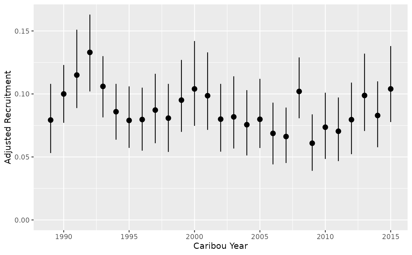
Recruitment for a ‘typical’ year
predict_recruitment_1 <- bb_predict_recruitment(recruitment, year = FALSE)
predict_recruitment_1
#> # A tibble: 1 × 6
#>   PopulationName CaribouYear Month estimate  lower  upper
#>   <fct>                <int> <int>    <dbl>  <dbl>  <dbl>
#> 1 A                       NA    NA   0.0868 0.0752 0.0972
Recruitment trend
predict_recruitment_trend <- bb_predict_recruitment_trend(recruitment)
bb_plot_year_trend_recruitment(predict_recruitment_trend)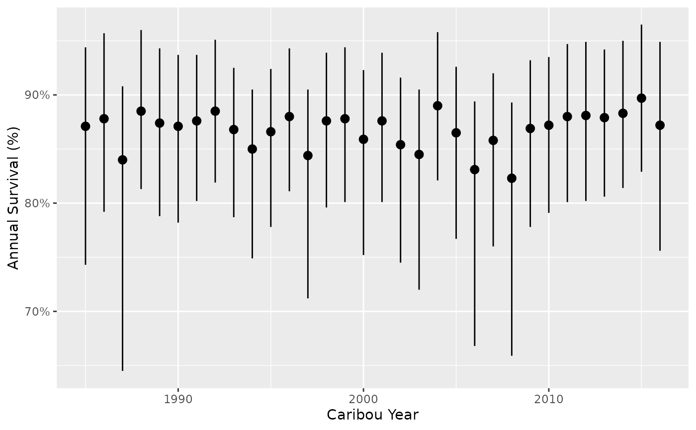
Survival by year for a ‘typical’ month
predict_survival <- bb_predict_survival(survival, year = TRUE, month = FALSE)
bb_plot_year_survival(predict_survival)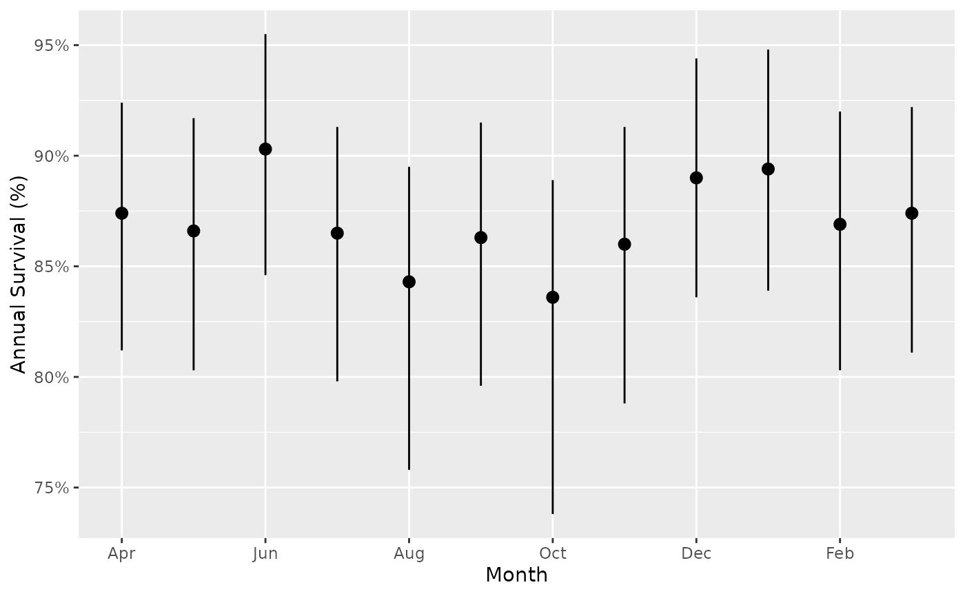
Survival by month for a ‘typical’ year
The estimates show annual survival, i.e., if that month lasted the duration of the year.
predict_survival_month <- bb_predict_survival(survival, year = FALSE, month = TRUE)
bb_plot_month_survival(predict_survival_month)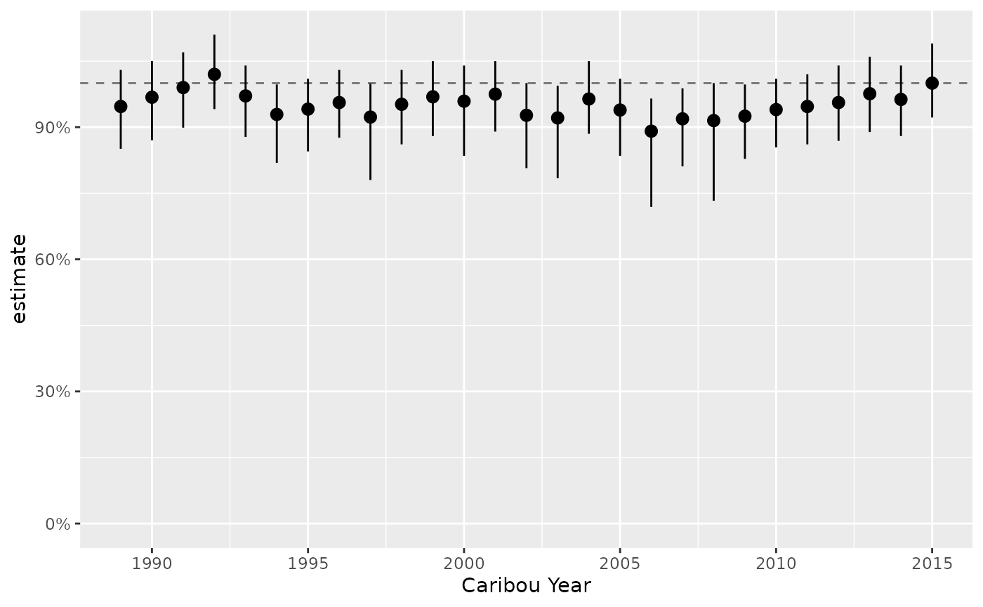
Population Growth
A user can predict population growth (lambda) with
bb_predict_growth(). The survival and recruitment models
fit in the previous steps are used as input. It is important to ensure
that survival and recruitment outputs share the same biological year
(i.e., ‘caribou year’), which is set with the year_start
argument in bb_fit_survival() and
bb_fit_recruitment(). Details on how lambda is calculated
can be found in the analytical
methods article.
predict_lambda <- bb_predict_growth(survival = survival, recruitment = recruitment)
#> Filtering to shared population and year combinations. CaribouYears in survival only: 1985, 1986, 1987, 1988, 2016.

bb_plot_year_growth(predict_lambda) +
  ggplot2::scale_y_continuous(labels = scales::percent)
#> Scale for y is already present.
#> Adding another scale for y, which will replace the existing scale.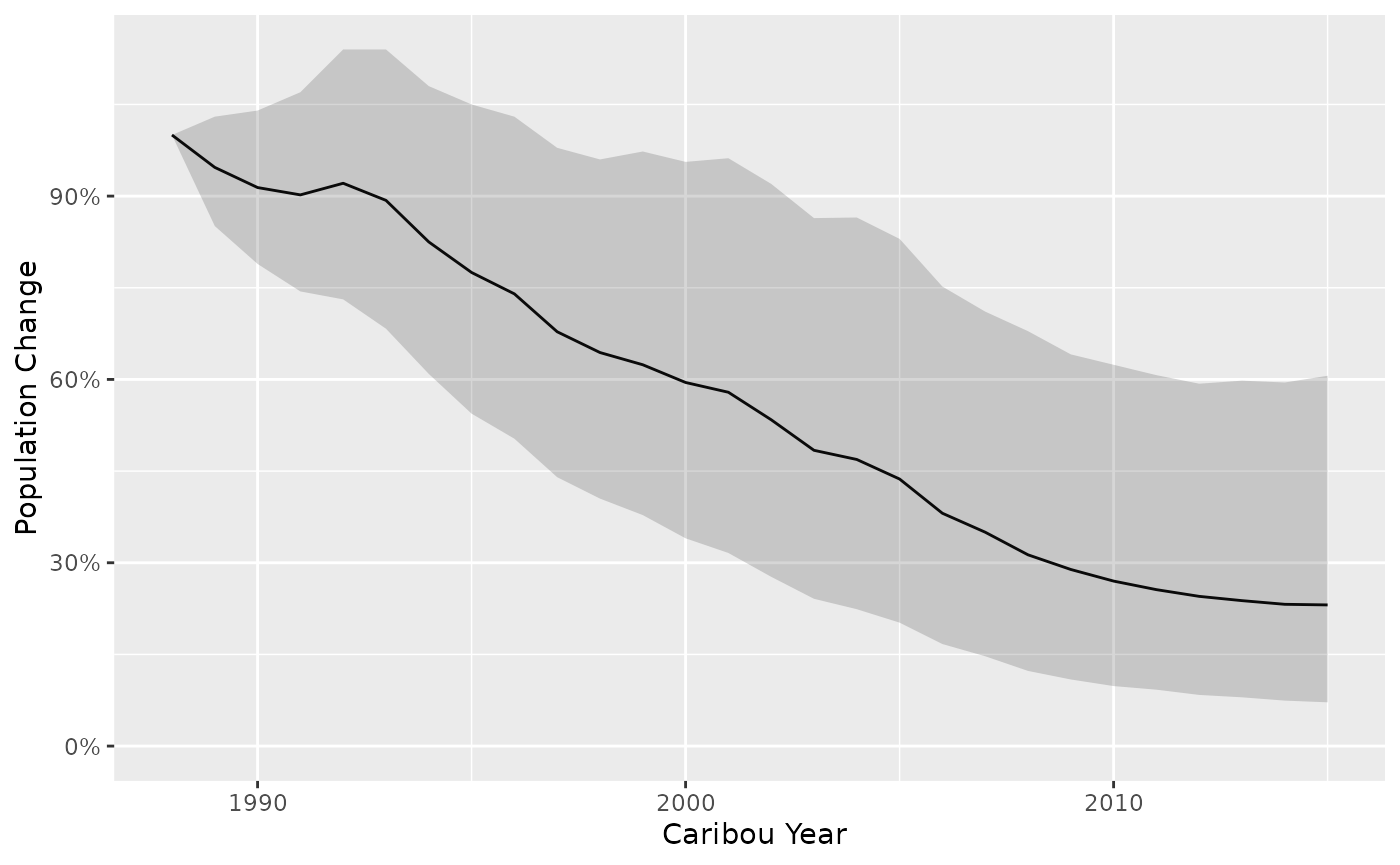
Population change (%) is calculated with uncertainty as the cumulative product of population growth.
predict_change <- bb_predict_population_change(survival = survival, recruitment = recruitment)
#> Filtering to shared population and year combinations. CaribouYears in survival only: 1985, 1986, 1987, 1988, 2016.
bb_plot_year_population_change(predict_change)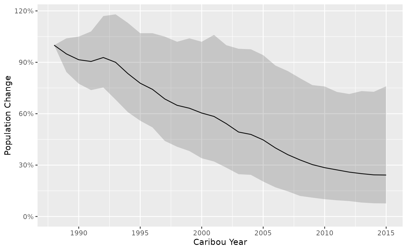
Multi-Population Analysis
bboutools can fit models to data from multiple
populations simultaneously. The function bb_fit_survival()
auto-detects multiple populations from the PopulationName
column.
survival_multi <- bb_fit_survival(bboudata::bbousurv_multi, allow_missing = TRUE, quiet = TRUE)Prediction plots are automatically faceted by population.
pred_multi <- bb_predict_survival(survival_multi)
bb_plot_year_survival(pred_multi)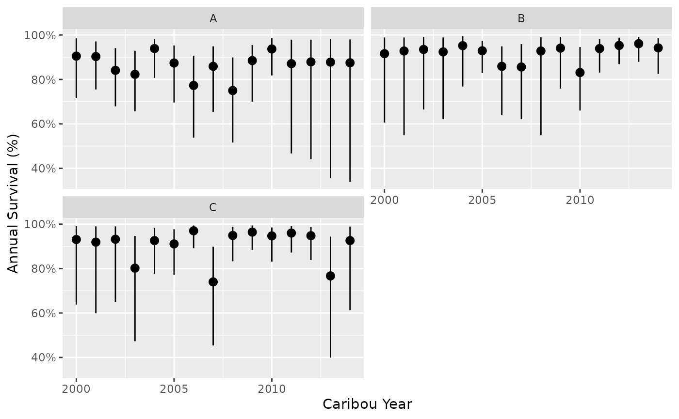
The default faceting can be overridden since all plot functions
return ggplot2 objects.
See the extensions article for more information on multi-population analysis, aggregate annual survival data, predicting unobserved years and other extensions.
Maximum Likelihood
Maximum Likelihood (ML) models can be fit using the
bb_fit_recruitment_ml() and
bb_fit_survival_ml() functions. These functions take a few
seconds to execute because Nimble must compile the model into C++ code.
See the Nimble
documentation for more information and comparison to TMB. Similar to
Bayesian model fits, generic functions (e.g., tidy(),
glance() and augment()) work on ML fit objects
(class ‘bboufit_ml’).
recruitment_ml <- bb_fit_recruitment_ml(bboudata::bbourecruit_a, year_start = 4, year_trend = TRUE, quiet = TRUE)
glance(recruitment_ml)
#> # A tibble: 1 × 4
#>       n     K loglik converged
#>   <int> <int>  <dbl> <lgl>
#> 1    27     3  -90.1 TRUE
survival_ml <- bb_fit_survival_ml(bboudata::bbousurv_a, year_start = 4, quiet = TRUE)The ML estimates are comparable to estimates derived from the equivalent Bayesian models above. In general, ML models can be interpreted as Bayesian models with uninformative (e.g., uniform) priors (McElreath 2016).
tidy(recruitment_ml, include_random_effects = FALSE)
#> # A tibble: 29 × 4
#>    term          estimate lower upper
#>    <chr>            <dbl> <dbl> <dbl>
#>  1 b0[1]            -1.43 -1.43 -1.43
#>  2 bAnnual[1, 1]     0     0     0
#>  3 bAnnual[2, 1]     0     0     0
#>  4 bAnnual[3, 1]     0     0     0
#>  5 bAnnual[4, 1]     0     0     0
#>  6 bAnnual[5, 1]     0     0     0
#>  7 bAnnual[6, 1]     0     0     0
#>  8 bAnnual[7, 1]     0     0     0
#>  9 bAnnual[8, 1]     0     0     0
#> 10 bAnnual[9, 1]     0     0     0
#> # ℹ 19 more rows
tidy(survival_ml, include_random_effects = FALSE)
#> # A tibble: 4 × 4
#>   term     estimate  lower upper
#>   <chr>       <dbl>  <dbl> <dbl>
#> 1 b0[1]       4.45  4.45   4.45
#> 2 bYear[1]    0     0      0
#> 3 sAnnual     0.336 0.133  0.846
#> 4 sMonth      0.238 0.0722 0.787
There is functionality in bboutools to generate
predictions (i.e., derived parameters) from ML models. However, there is
no functionality to get confidence intervals on predictions. This is a
more straightforward task with Bayesian models.
bb_predict_survival(survival_ml)
#> # A tibble: 32 × 6
#>    PopulationName CaribouYear Month estimate lower upper
#>    <fct>                <int> <int>    <dbl> <dbl> <dbl>
#>  1 A                     1985    NA    0.873    NA    NA
#>  2 A                     1986    NA    0.883    NA    NA
#>  3 A                     1987    NA    0.83     NA    NA
#>  4 A                     1988    NA    0.89     NA    NA
#>  5 A                     1989    NA    0.875    NA    NA
#>  6 A                     1990    NA    0.871    NA    NA
#>  7 A                     1991    NA    0.878    NA    NA
#>  8 A                     1992    NA    0.891    NA    NA
#>  9 A                     1993    NA    0.868    NA    NA
#> 10 A                     1994    NA    0.842    NA    NA
#> # ℹ 22 more rows
growth <- bb_predict_growth(survival_ml, recruitment_ml)
#> Filtering to shared population and year combinations. CaribouYears in survival only: 1985, 1986, 1987, 1988, 2016.
bb_plot_year_growth(growth)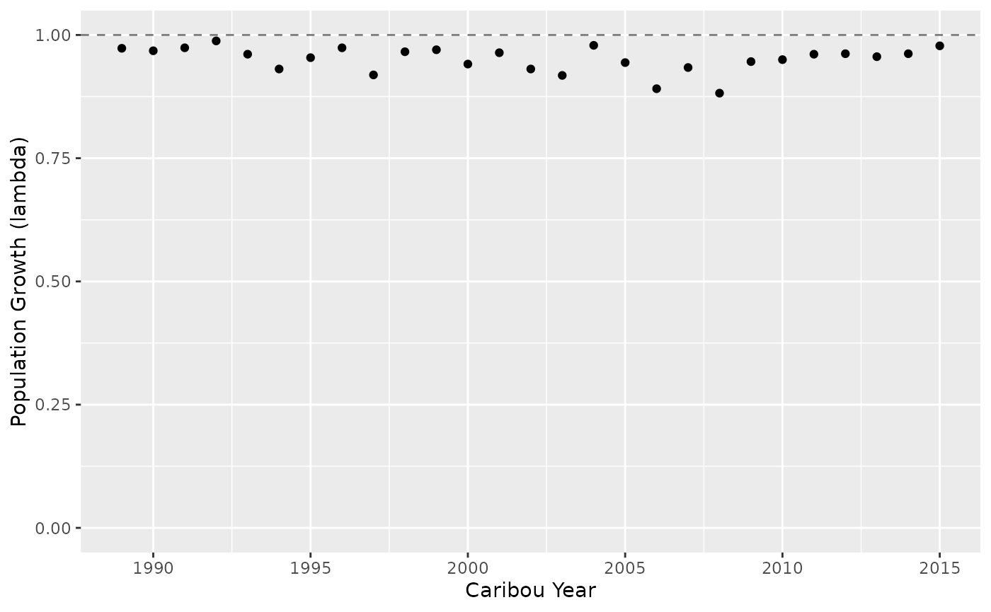
ML models do not currently support multi-population analysis,
unobserved year predictions (allow_missing) or prior-only
sampling. These features are available only with the Bayesian fitting
functions.
Note that ML models can struggle to converge when there are sparse
data, especially with a fixed year effect. If these issues arise, the
user can try estimating year as a random effect, continuous effect
(year_trend), or fitting a Bayesian model.
Another possible source of convergence issues is initial values. By
default, bboutools sets initial values based on the default
priors used for parameters in the Bayesian models. The user can replace
initial values for parameters using inits.
inits_ml <- bb_fit_recruitment_ml(bboudata::bbourecruit_a, inits = c(b0 = 1, sAnnual = 0.3))Understanding bboufit objects
The bb_fit_survival() and
bb_fit_recruitment() functions use a Bayesian approach and
return objects that inherit from class bboufit.
Objects of class bboufit have four elements:
-
model- the compiled Nimble model as created bynimble::nimbleModel().
-
model_code- the model code in text format.
-
samples- the MCMC samples generated fromnimble::runMCMC()converted to an object of classmcmcr.
-
data- the survival or recruitment data provided.
These are the raw materials for any further exploration or analysis.
For example, view trace and density plots with
plot(fit$samples).
See mcmcr
and mcmcderive
for working with mcmcr objects, or convert samples to an
object of class mcmc.list, e,g, with
coda::as.mcmc.list for working with the coda R package.
The bb_fit_survival_ml() and
bb_fit_recruitment_ml() functions use a Maximum Likelihood
approach and return objects that inherit from class
bboufit_ml.
Objects of class bboufit_ml have five elements:
-
model- the Nimble model as created bynimble::nimbleModel().
-
model_code- the model code in text format.
-
mle- the Maximum Likelihood output as created by model$findMLE(). -
summary- the summary of the Maximum Likelihood output as created bymodel$summary(mle).
-
data- the survival or recruitment data provided.
See nimble for how to work with nimble model objects and Maximum Likelihood output.