Getting Started with bisonpictools

bisonpictools is an R package to facilitate the visualization and analysis of camera trap data for wood bison herds. The package includes functions to check the correct formatting of data, visualize the data, manipulate and analyse the data using a complex custom-built Bayesian model, and generate and plot predictions of abundances, survival and fecundity rates, and population ratios.

Installation

To install the latest development version of bisonpictools, execute the following code in the RStudio console.

install.packages("remotes")
remotes::install_github("poissonconsulting/bisonpictools")

bisonpic Suite

bisonpictools is part of the bisonpic suite of tools. Other packages in this suite include:

Getting Help

To get additional information on a particular function just type ? followed by the name of the function in the R console. For example, ?bpt_analyse() brings up the R documentation for the bisonpictools analysis function.

For more information on using R the reader is referred to R for Data Science (Wickham and Grolemund 2016).

If you discover a bug in bisonpictools please file an issue with a reprex (reproducible example).

Data

The easiest way to prepare the data for use with the bisonpictools functions is to download the templated excel spreadsheet from the shinybisonpic website. Click the Download Template button, and populate each sheet with your data.

event_data contains the camera trap event data, including the date and time of each event, location of the camera trap, and the number of individuals in each class
location_data contains the coordinates of the camera traps
census_data contains population estimates of the population from aerial surveys, and the date of the surveys
- specifically, this should be an estimate of the entire population size, not a minimum count
proportion_calf_data contains estimates of the proportion of calves in the population from aerial surveys, and the date of the surveys

Data Visualization

Using the RStudio Console

Functions from bisonpictools can be run in the RStudio console. The bpt_plot_ratios() function plots the ratios of various sex-age classes over time. The user needs to provide the event and location data, as well as vectors of classes to form the numerator and denominator of the ratio.

(1) Read in data from the populated excel template

# Change `dir` to the file path of the populated excel template on your computer
dir <- "myfilepath.xlsx"
# Install readxl to read the excel spreadsheet into R
remotes::install_github("readxl")
# Read each sheet into R
location_data <- readxl::read_xlsx(dir, sheet = "location")
event_data <- readxl::read_xlsx(dir, sheet = "event")
census_data <- readxl::read_xlsx(dir, sheet = "census")
proportion_calf_data <- readxl::read_xlsx(dir, sheet = "proportion_calf")

(2) Produce ratio plots

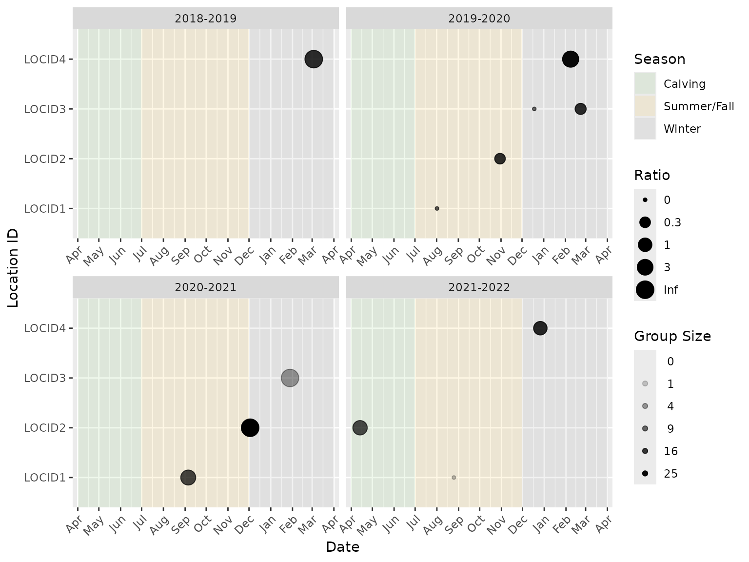
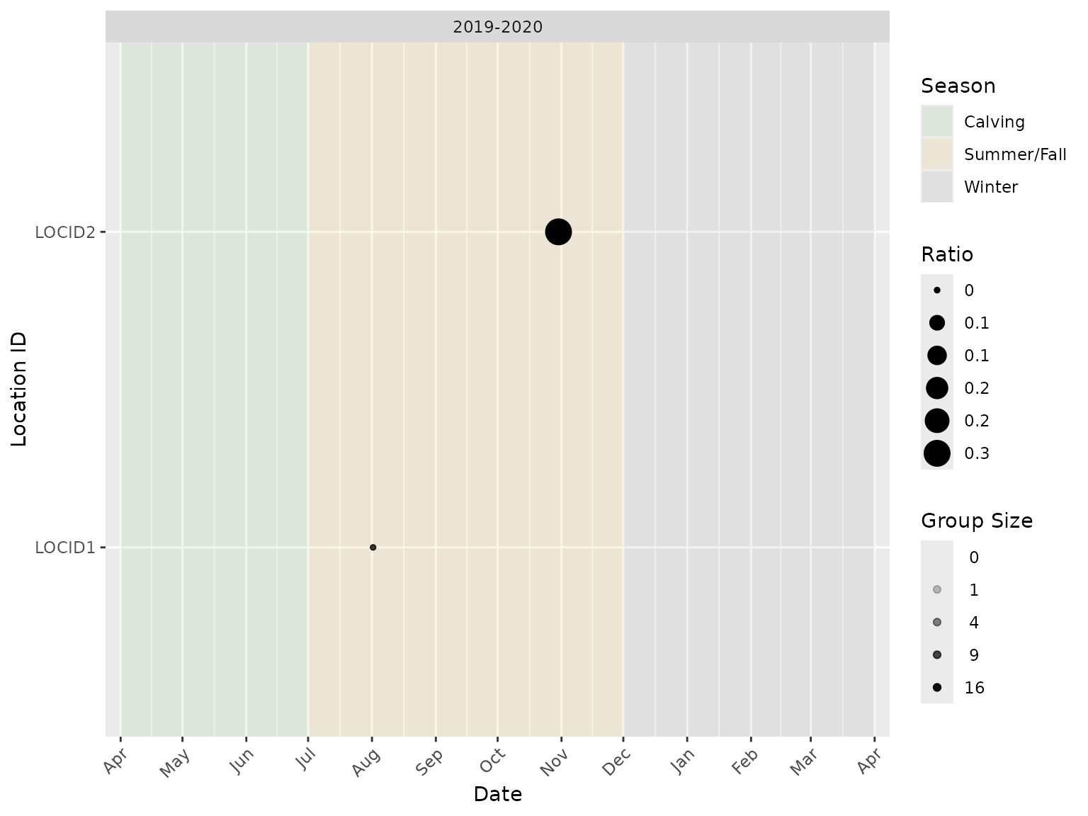
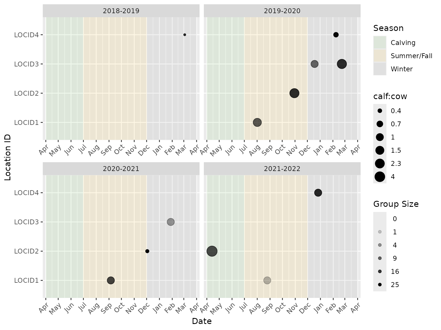
Data checks are completed before the analysis is run to ensure they are in the correct format. In the plot, each point represents an event. The size (area) of the point indicates the ratio while the opacity of the point indicates the number of individuals in the group.

Note that a ratio value of “Inf” (infinity) indicates that the group in a particular camera trap event has no individuals in the denominator class. For example, if plotting the calf:cow ratio, a ratio value of “Inf” would represent an event with one or more calves and no cows. Similarly, a ratio of “0” indicates that the ratio in a particular camera trap event has no individuals in the numerator class. For the calf:cow ratio example, this would represent an event with one or more cows and no calves.

For example, the female calf:male calf ratio plotted over all years and locations from example data:

library(bisonpictools)
bpt_plot_ratios(
  event_data,
  location_data,
  numerator = "f0",
  denominator = "m0"
)

It is also possible to subset the data to include one or more camera trap locations and/or study years:

bpt_plot_ratios(
  event_data,
  location_data,
  numerator = "f0",
  denominator = "m0",
  study_years = "2019-2020",
  locations = c("LOCID1", "LOCID2")
)

Several age/sex classes can be combined to plot ratios of interest. For example, the next code chunk plots the calf:(cow + calf) ratio.

The label for the ratio legend can be changed from the default (“Ratio”), to more specific label, using the ratio_name argument.

bpt_plot_ratios(
  event_data,
  location_data,
  numerator = c("f0", "m0", "u0"),
  denominator = c("fa"),
  ratio_name = "calf:cow"
)

`shinybisonpic`

The shinybisonpic Shiny app can be used to explore the locations of camera traps and the the ratios of different classes of wood bison in camera trap observations in a user-friendly manner. Refer to the user guide for more information on how to use the shinybisonpic app.

Data Analysis

Using the RStudio Console

(1) Read in data from the populated excel template

# Change `dir` to the file path of the populated excel template on your computer
dir <- "myfilepath.xlsx"
# Install readxl to read the excel spreadsheet into R
remotes::install_github("readxl")
# Read each sheet into R
location_data <- readxl::read_xlsx(dir, sheet = "location")
event_data <- readxl::read_xlsx(dir, sheet = "event")
census_data <- readxl::read_xlsx(dir, sheet = "census")
proportion_calf_data <- readxl::read_xlsx(dir, sheet = "proportion_calf")

(2) Run the analysis

This uses the bpt_analyse() function. Data checks are completed before the analysis is run to ensure they are in the correct format. Informative error messages will print to the console if the data do not follow the required format. The following arguments control the number of MCMC chains, number of iterations, and the thinning rate of the model:

analysis_mode controls the number of iterations and chains in the model run:
- "debug" is used for printing out the errors if the model does not sample (10 iterations from 2 chains),
- "quick" is used for running through a quick run of the model for demonstration purposes (10 iterations from 2 chains),
- "report" is the default and is used for the full analysis (500 iterations from 3 chains).
nthin controls the thinning of the MCMC samples:
- nthin = 1L saves every sample; use this for "debug" and "quick" modes,
- nthin = 10L saves every $10^{th}$ sample, and is the detault; use this for "report" mode,
- increase nthin by 5 if the model does not converge in “report” mode.

It is recommended to:

Run the model in analysis_mode = "quick" mode with a thinning rate of nthin = 1L to ensure the model samples correctly.
If there were no errors in step 1, proceed by running the model in analysis_mode = "report" with a thinning rate of nthin = 10L, to achieve convergence. Ensure the table output by the model has TRUE in the “converged” column. If the model did not converge, increase nthin by 5, and re-run the model.
If there were errors in step 1, proceed instead by running the model in analysis_mode = "debug" with a thinning rate of nthin = 1L to print informative error messages.

# Start by running once on "quick" mode, with a thinning rate of 1
analysis <- bpt_analyse(
  event_data = event_data,
  location_data = location_data,
  census_data = census_data,
  proportion_calf_data = proportion_calf_data,
  nthin = 1L,
  analysis_mode = "quick"
)

# If no errors appear, run the model on "report" mode, with a thinning rate of 10
analysis <- bpt_analyse(
  event_data = event_data,
  location_data = location_data,
  census_data = census_data,
  proportion_calf_data = proportion_calf_data,
  nthin = 10L,
  analysis_mode = "report"
)

# If errors do appear, run the model on "debug" mode, which will provide
# informative error messages
analysis <- bpt_analyse(
  event_data = event_data,
  location_data = location_data,
  census_data = census_data,
  proportion_calf_data = proportion_calf_data,
  nthin = 1L,
  analysis_mode = "debug"
)

(3) Check that the model converged

In "quick" or "debug" mode, convergence is not expected. In "report" mode, convergence is expected. See the converged column in the table printed after bpt_analyse() is run to assess whether or not the analysis converged. If it says TRUE, the model converged. If it says FALSE, the model did not converge.

This is an example of a model run in “quick” mode that did not converge (i.e., the “converged” column reads FALSE).

#> # A tibble: 1 × 8
#>       n     K nchains niters nthin   ess  rhat converged
#>   <int> <int>   <int>  <int> <int> <int> <dbl> <lgl>    
#> 1    11    57       2     10     1     7  1.97 FALSE

(4) Coefficient table

Use the bpt_coefficient_table() function to print out the estimated parameters from the model run.

coef <- bpt_coefficient_table(analysis)
print(coef)
#> # A tibble: 57 × 5
#>    term                           estimate    lower  upper svalue
#>    <term>                            <dbl>    <dbl>  <dbl>  <dbl>
#>  1 bEtaSummerFall                    0.232  0.00955  0.753  4.39 
#>  2 bEtaWin                           0.101  0.00114  0.484  4.39 
#>  3 bFecundityReproductiveFA          1.94   1.63     2.69   4.39 
#>  4 bInitialMortalityCalfAnnual[1]   -3.75  -5.78    -2.12   4.39 
#>  5 bInitialMortalityCalfAnnual[2]   -4.56  -7.45    -2.35   4.39 
#>  6 bInitialMortalityCalfAnnual[3]   -2.87  -7.46    -1.60   4.39 
#>  7 bInitialMortalityCalfAnnual[4]   -1.09  -6.11     3.64   0.485
#>  8 bKmWeekSummerFall                 2.22   0.266    4.42   4.39 
#>  9 bKmWeekWin                        1.93   1.21     2.63   4.39 
#> 10 bMAProportion[1]                  0.440  0.258    0.582  4.39 
#> # ℹ 47 more rows

(5) Save the analysis object

Ensure that the analysis object is saved once the model finishes running. The bpt_save_analysis() function saves the analysis to the desired file path.

# Save the analysis object.
# Change the file path to the desired directory (does not require a file extension)
bpt_save_analysis(analysis, file = "file_path/analysis")

To load the analysis object back into R, use the complimentary function, bpt_load_analysis(), using the same file path it was saved to above.

# Load analysis object if not still in the environment, using the same file path
# it was saved to in step (4) above.
analysis <- bpt_load_analysis("file_path/analysis")

(6) Make predictions

Predictions of the stage-wise and total abundances, survival and fecundity rates, and select ratios are derived from the posterior distributions of the estimated parameters. Use the functions with the bpt_predict prefix to generate the predictions.

# Predict total abundance
bpt_predict_abundance_total(analysis)
#> # A tibble: 4 × 4
#>   annual    estimate lower upper
#>   <fct>        <dbl> <dbl> <dbl>
#> 1 2018-2019     211.  182.  244.
#> 2 2019-2020     225.  205.  252.
#> 3 2020-2021     254.  230.  280.
#> 4 2021-2022     295.  258.  311.

# Predicts abundance by class:
bpt_predict_abundance_class(analysis)
#> # A tibble: 32 × 5
#>    annual    class estimate lower upper
#>    <fct>     <chr>    <dbl> <dbl> <dbl>
#>  1 2018-2019 F0        41.3 27.8   63.3
#>  2 2019-2020 F0        32.6 26.2   36.9
#>  3 2020-2021 F0        40.9 35.3   43.0
#>  4 2021-2022 F0        44.4 35.0   47.6
#>  5 2018-2019 F1        17.0  6.53  43.2
#>  6 2019-2020 F1        20.1 12.4   31.6
#>  7 2020-2021 F1        17.7  8.95  23.2
#>  8 2021-2022 F1        25.0 20.2   30.2
#>  9 2018-2019 FA        64.0 51.8   82.0
#> 10 2019-2020 FA        80.6 65.1   91.5
#> # ℹ 22 more rows

# Predicts survival rates by class:
bpt_predict_survival(analysis)
#> # A tibble: 24 × 5
#>    annual    class estimate  lower upper
#>    <fct>     <fct>    <dbl>  <dbl> <dbl>
#>  1 2018-2019 F0       0.460 0.366  0.648
#>  2 2019-2020 F0       0.510 0.312  0.682
#>  3 2020-2021 F0       0.587 0.469  0.701
#>  4 2021-2022 F0       0.324 0.0146 0.635
#>  5 2018-2019 M0       0.445 0.196  0.679
#>  6 2019-2020 M0       0.570 0.414  0.760
#>  7 2020-2021 M0       0.507 0.406  0.643
#>  8 2021-2022 M0       0.364 0.0174 0.677
#>  9 2018-2019 F1       0.873 0.679  0.932
#> 10 2019-2020 F1       0.850 0.726  0.919
#> # ℹ 14 more rows

# Predicts fecundity rate and proportion of reproductive cows:
bpt_predict_fecundity(analysis)
#> # A tibble: 2 × 4
#>   rate                            estimate lower upper
#>   <chr>                              <dbl> <dbl> <dbl>
#> 1 Fecundity                          0.875 0.836 0.936
#> 2 Proportion of Reproductive Cows    0.965 0.888 0.996

# Predicts population ratios:
bpt_predict_ratios(analysis)
#> # A tibble: 28 × 5
#>    annual    ratio   estimate lower upper
#>    <fct>     <fct>      <dbl> <dbl> <dbl>
#>  1 2018-2019 M0:F0      0.802 0.384 1.35 
#>  2 2019-2020 M0:F0      1.13  0.895 1.63 
#>  3 2020-2021 M0:F0      0.847 0.647 1.26 
#>  4 2021-2022 M0:F0      1.12  0.668 2.40 
#>  5 2018-2019 M1:F1      1.14  0.439 3.28 
#>  6 2019-2020 M1:F1      0.771 0.393 1.28 
#>  7 2020-2021 M1:F1      1.08  0.938 1.72 
#>  8 2021-2022 M1:F1      0.935 0.523 1.45 
#>  9 2018-2019 Calf:FA    0.590 0.367 0.758
#> 10 2019-2020 Calf:FA    0.464 0.297 0.591
#> # ℹ 18 more rows

(7) Plot Predictions

The bpt_plot_predictions() function can be used to visualize the predictions.

# Plot predicted abundances by class
bpt_plot_predictions(analysis, prediction = "abundance-class")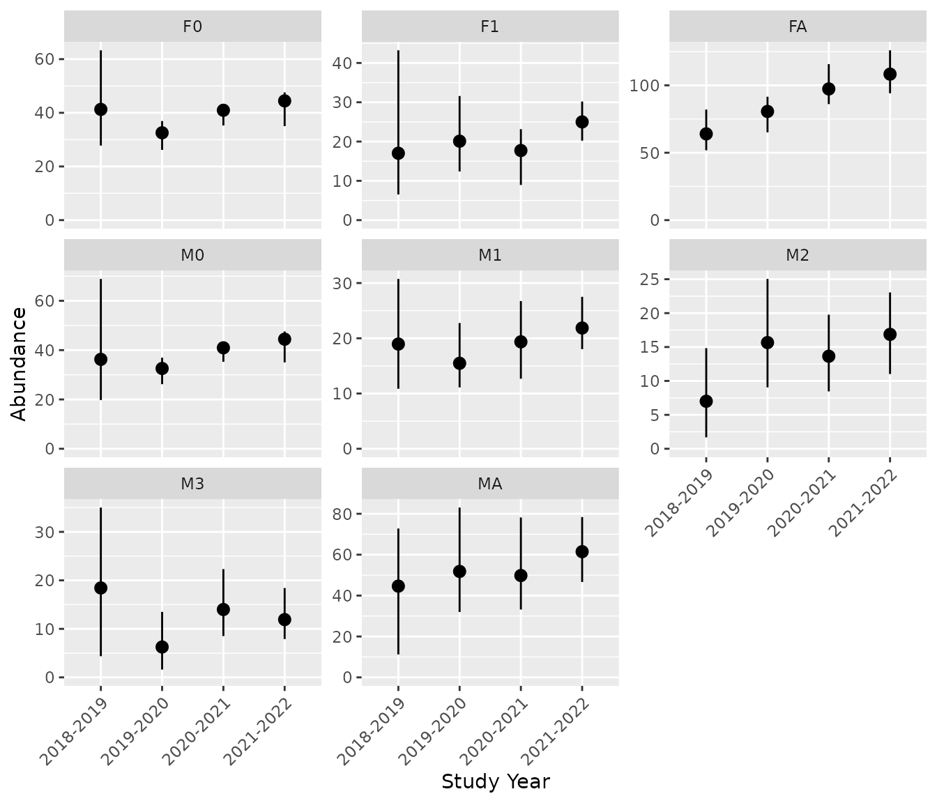

# Plot total abundance
bpt_plot_predictions(analysis, prediction = "abundance-total")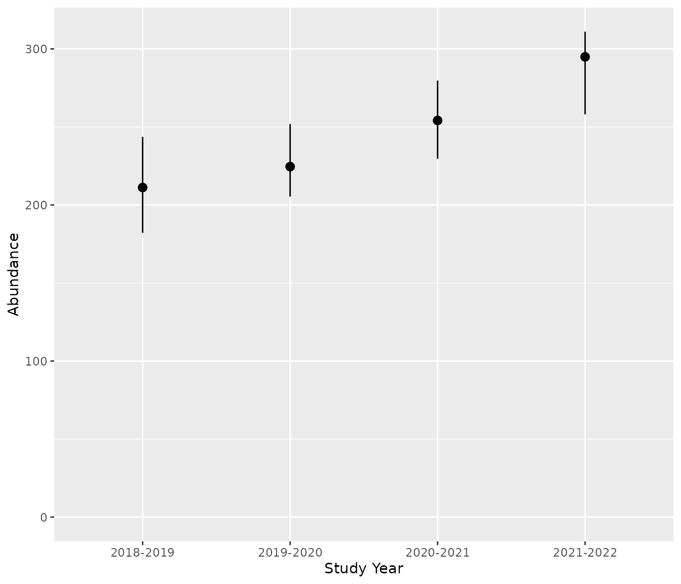

# Plot survival rates
bpt_plot_predictions(analysis, prediction = "survival")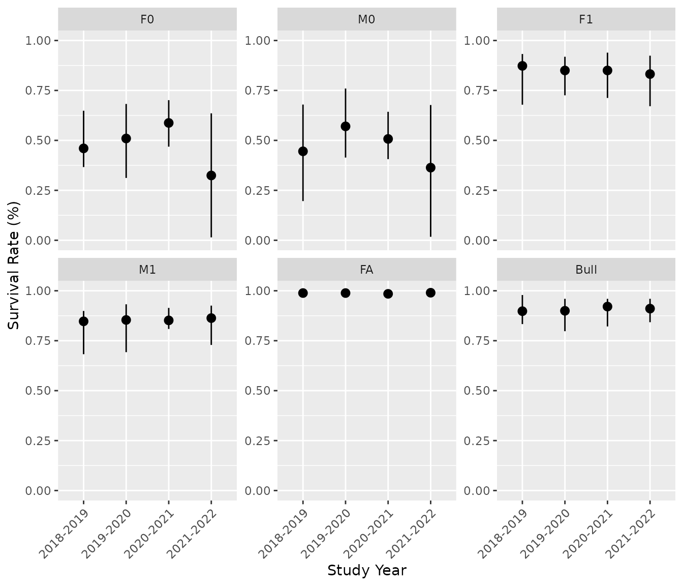

# Plot fecundity rates
bpt_plot_predictions(analysis, prediction = "fecundity")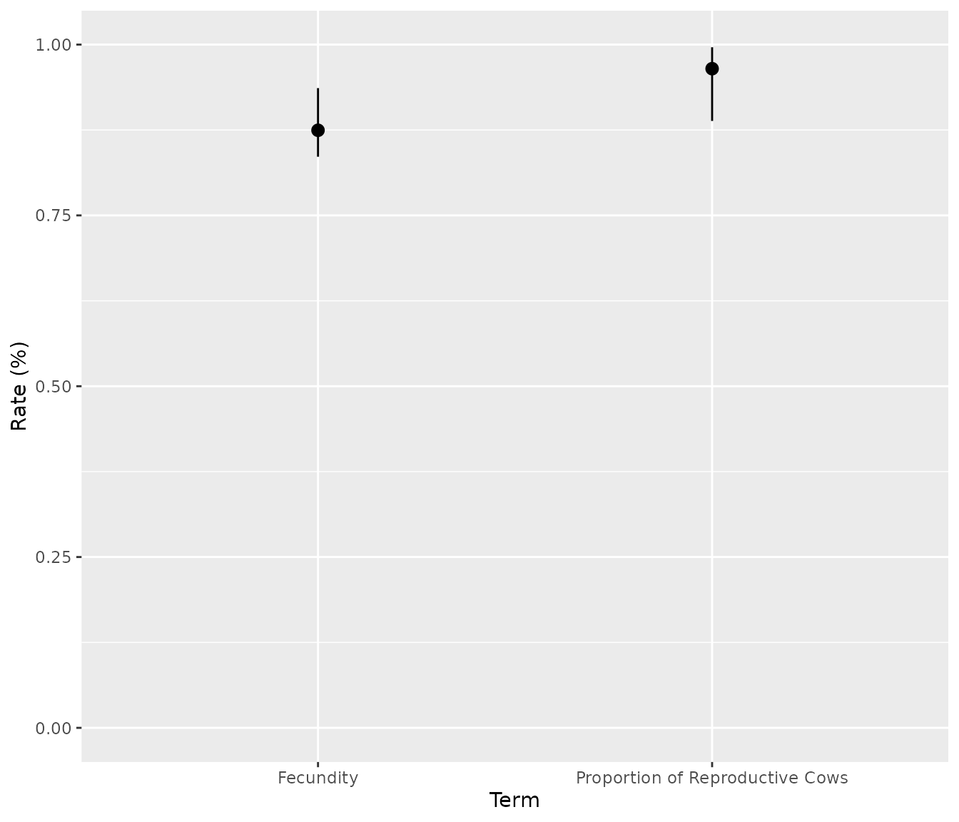

# Plot ratios
bpt_plot_predictions(analysis, prediction = "ratios")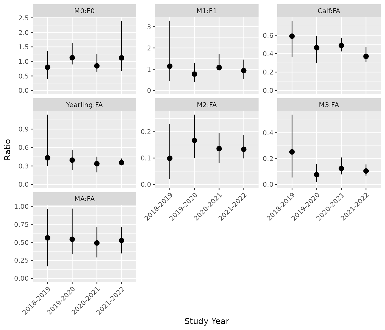

`runbisonpic`

Alternatively, launch the local data analysis app by running the following lines of code in the RStudio console.

# Install `runbisonpic`
remotes::install_github("poissonconsulting/runbisonpic")
# Launch local app
runbisonpic::launch_runbisonpic()

See the user guide for more guidance on how to use the runbisonpic app.

Going beyond `bisonpictools`

The analysis object is a list that contains the model code, mcmc samples (class mcmcr), and other meta-data used to fit the model. The user can interact directly with the mcmc samples using packages such as mcmcr and mcmcderive to derive other quantities of interest.

References

Wickham, Hadley, and Garrett Grolemund. 2016. R for Data Science: Import, Tidy, Transform, Visualize, and Model Data. First edition. Sebastopol, CA: O’Reilly. https://r4ds.had.co.nz.

Licensing

Licensed under the Apache License, Version 2.0 (the “License”); you may not use this file except in compliance with the License. You may obtain a copy of the License at

http://www.apache.org/licenses/LICENSE-2.0

Unless required by applicable law or agreed to in writing, software distributed under the License is distributed on an “AS IS” BASIS, WITHOUT WARRANTIES OR CONDITIONS OF ANY KIND, either express or implied. See the License for the specific language governing permissions and limitations under the License.

Installation

bisonpic Suite

Getting Help

Data

Data Visualization

Using the RStudio Console

(1) Read in data from the populated excel template

(2) Produce ratio plots

shinybisonpic

Data Analysis

Using the RStudio Console

(1) Read in data from the populated excel template

(2) Run the analysis

(3) Check that the model converged

(4) Coefficient table

(5) Save the analysis object

(6) Make predictions

(7) Plot Predictions

runbisonpic

Going beyond bisonpictools

References

Licensing

`shinybisonpic`

`runbisonpic`

Going beyond `bisonpictools`