Prediction with predict() and Related Functions

predict.mb_analysis() summarizes the posterior predictive distribution of a fitted Bayesian model at new covariate values, returning a tidy data frame with point estimates and compatibility limits. This vignette covers:

Covariate grids built with the newdata helpers.
Scalar quantities from new_expr.
Random-effect zeroing control.
Reference data and effect sizes, e.g., for proportional change.
Predicting for an unobserved level to include amongst-level variation.
Overriding new_expr and injecting constants for ad-hoc derived quantities.
Group-level summaries with mcmc_derive_data().
Combining across analyses with combine_samples() for joining and summarizing samples from independent fits.
Scalar derived quantities with mcmc_derive() and arithmetic on raw mcmcr posteriors.
Cheat sheet mapping common goals to tools.

library(embr)
library(smbr2)
library(newdata)
library(mcmcr)
library(mcmcderive)
library(dplyr)
library(ggplot2)

Setup: fit demo model

A simple example fish count model is fit with Stan (via cmdstanr and smbr2). The simulated data has 5 sites × 5 years × 2 treatments, with an unbalanced design (i.e., not all sites have all years with data).

count_code <- "
data {
  int<lower=2> nObs;
  int<lower=1> nsite;
  int<lower=1> nannual;
  int<lower=1> ntreatment;
  array[nObs] int<lower=1> site;
  array[nObs] int<lower=1> annual;
  array[nObs] int<lower=1> treatment;
  vector[nObs] temperature;
  array[nObs] int<lower=0> count;
}
parameters {
  real bIntercept;
  vector[ntreatment - 1] bTreatment_dev;
  real bTemp;
  real<lower=0> sSite;
  real<lower=0> sAnnual;
  real<lower=0> bPhi;
  vector[nsite] z_bSite;
  vector[nannual] z_bAnnual;
}
model {
  vector[nsite] bSite = z_bSite * sSite;
  vector[nannual] bAnnual = z_bAnnual * sAnnual;
  vector[ntreatment] bTreatment;
  bTreatment[1] = 0;
  for (k in 2:ntreatment) bTreatment[k] = bTreatment_dev[k - 1];

  vector[nObs] log_eCount;
  for (i in 1:nObs) {
    log_eCount[i] = bIntercept + bTreatment[treatment[i]] +
                    bTemp * temperature[i] + bSite[site[i]] +
                    bAnnual[annual[i]];
  }

  bIntercept ~ normal(0, 5);
  bTreatment_dev ~ normal(0, 5);
  bTemp ~ normal(0, 5);
  sSite ~ exponential(1);
  sAnnual ~ exponential(1);
  bPhi ~ gamma(2, 0.5);
  to_vector(z_bSite) ~ std_normal();
  to_vector(z_bAnnual) ~ std_normal();

  count ~ neg_binomial_2_log(log_eCount, bPhi);
}
"

count_model <- model(
  code = count_code,
  new_expr = {
    bSite <- z_bSite * sSite
    bAnnual <- z_bAnnual * sAnnual
    bTreatment <- c(0, bTreatment_dev)
    eBaseCount <- exp(bIntercept)
    eRestoredEffect <- exp(bTreatment_dev[1])
    for (i in 1:nObs) {
      log(eCount[i]) <- bIntercept +
        bTreatment[treatment[i]] +
        bTemp * temperature[i] +
        bSite[site[i]] +
        bAnnual[annual[i]]
      prediction[i] <- eCount[i]
      fit[i] <- eCount[i]
      unobserved[i] <- exp(
        bIntercept +
          bTreatment[treatment[i]] +
          bTemp * temperature[i] +
          rnorm(1, 0, sSite) +
          rnorm(1, 0, sAnnual)
      )
      log_lik[i] <- log_lik_neg_binom(count[i], eCount[i], bPhi)
    }
  },
  new_expr_vec = TRUE,
  select_data = list(
    count = 1L,
    site = factor("a"),
    annual = factor("a"),
    treatment = factor("a"),
    `temperature*` = 1
  ),
  random_effects = list(
    z_bSite = "site",
    z_bAnnual = "annual"
  )
)

analysis <- analyse(
  count_model,
  data = data,
  stan_engine = "cmdstan-mcmc",
  nchains = 3L,
  niters = 500L,
  niters_warmup = 500L,
  seed = 42L,
  parallel = TRUE,
  quiet = TRUE,
  beep = FALSE
)
#> # A tibble: 1 × 11
#>       n     K nchains niters nthin   ess  rhat converged num_divergent
#>   <int> <int>   <int>  <int> <int> <int> <dbl> <lgl>             <dbl>
#> 1   132     6       3    500     1   414  1.00 FALSE                 0
#> # ℹ 2 more variables: max_treedepth <int>, ebfmi <dbl>

coef(analysis, include_constant = FALSE, simplify = TRUE) |>
  mutate(across(estimate:svalue, ~ signif(.x, 3)))
#> # A tibble: 6 × 5
#>   term           estimate  lower upper svalue
#>   <term>            <dbl>  <dbl> <dbl>  <dbl>
#> 1 bIntercept        3.69  2.99   4.32   10.6 
#> 2 bPhi              4.13  3.13   5.41   10.6 
#> 3 bTemp             0.109 0.0203 0.193   6.38
#> 4 bTreatment_dev    0.55  0.387  0.727  10.6 
#> 5 sAnnual           0.267 0.113  0.782  10.6 
#> 6 sSite             0.464 0.232  1.25   10.6

Default prediction

With no new_data, predict() returns predicted values for every row of the analysis dataset. This is pulled from the prediction[i] line in new_expr:

predict(analysis) |> head()
#> # A tibble: 6 × 9
#>   count site  annual treatment temperature estimate lower upper svalue
#>   <int> <fct> <fct>  <fct>           <dbl>    <dbl> <dbl> <dbl>  <dbl>
#> 1    55 a     1      control          14.7     51.4  38.4  69.0   10.6
#> 2    55 b     1      control          10.9     78.3  59.9 104.    10.6
#> 3    19 c     1      control          12.7     85.6  65.9 112.    10.6
#> 4    51 d     1      control          13.3     40.7  31.1  53.2   10.6
#> 5    11 a     2      control          12.8     31.4  23.7  42.4   10.6
#> 6    53 b     2      control          11.8     56.1  42.1  74.7   10.6

Covariate grids with the `newdata` helpers

Covariate grids can be generated with newdata::xnew_data(). Covariates not specified are held at a reference value: mean for continuous, first level for factors. For categorical fixed effects this is the literal first level; for random-effect factors at the first level, that random effect is zeroed by default — see Random-effect zeroing below.

Continuous covariate

By default, specifying the name of a continuous covariate will generate a sequence from min to max, with length 30. Notice factors (e.g., site) are held at the first level.

temp_data <- xnew_data(data, temperature)
head(temp_data)
#> # A tibble: 6 × 5
#>   count site  annual treatment temperature
#>   <int> <fct> <fct>  <fct>           <dbl>
#> 1    62 a     1      control          6.01
#> 2    62 a     1      control          6.41
#> 3    62 a     1      control          6.80
#> 4    62 a     1      control          7.19
#> 5    62 a     1      control          7.58
#> 6    62 a     1      control          7.98
nrow(temp_data)
#> [1] 30

pred_temp <- predict(analysis, new_data = temp_data)

head(pred_temp)
#> # A tibble: 6 × 9
#>   count site  annual treatment temperature estimate lower upper svalue
#>   <int> <fct> <fct>  <fct>           <dbl>    <dbl> <dbl> <dbl>  <dbl>
#> 1    62 a     1      control          6.01     29.2  14.6  59.5   10.6
#> 2    62 a     1      control          6.41     29.8  15.0  60.1   10.6
#> 3    62 a     1      control          6.80     30.4  15.4  60.9   10.6
#> 4    62 a     1      control          7.19     31.1  15.9  62.0   10.6
#> 5    62 a     1      control          7.58     31.7  16.2  63.0   10.6
#> 6    62 a     1      control          7.98     32.4  16.4  63.6   10.6

plot_ribbon(pred_temp, temperature) +
  labs(y = "Expected count", x = "Temperature (scaled)")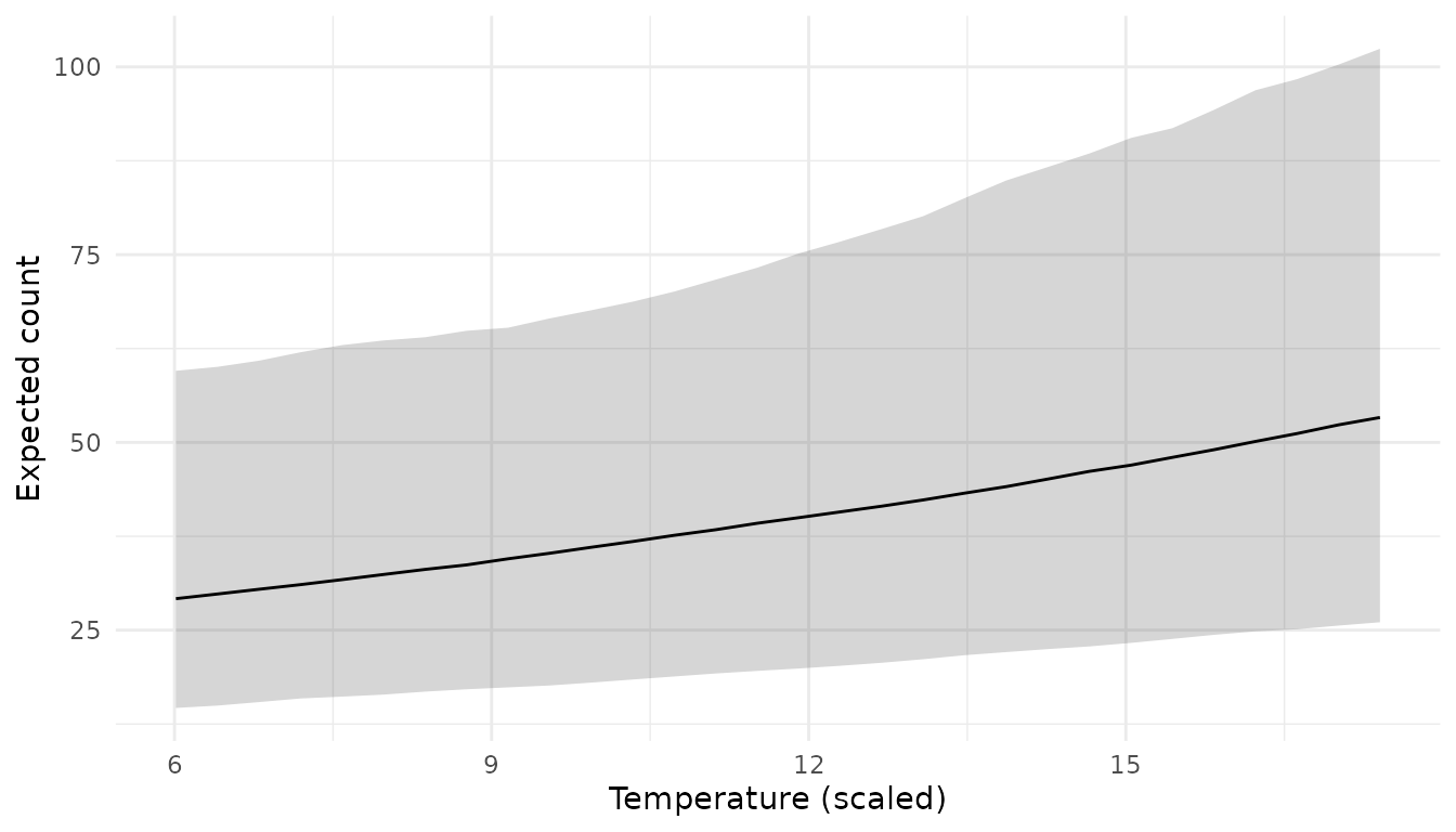

Specific values via `xnew_seq()` or with `=`

xnew_data(data, xnew_seq(temperature, length_out = 5)) |>
  predict(analysis, new_data = _)
#> # A tibble: 5 × 9
#>   count site  annual treatment temperature estimate lower upper svalue
#>   <int> <fct> <fct>  <fct>           <dbl>    <dbl> <dbl> <dbl>  <dbl>
#> 1    62 a     1      control          6.01     29.2  14.6  59.5   10.6
#> 2    62 a     1      control          8.86     33.9  17.2  65.0   10.6
#> 3    62 a     1      control         11.7      39.6  19.8  74.1   10.6
#> 4    62 a     1      control         14.6      45.9  22.7  88.0   10.6
#> 5    62 a     1      control         17.4      53.3  26.1 102.    10.6

xnew_data(data, temperature = 10) |>
  predict(analysis, new_data = _)
#> # A tibble: 1 × 9
#>   count site  annual treatment temperature estimate lower upper svalue
#>   <int> <fct> <fct>  <fct>           <dbl>    <dbl> <dbl> <dbl>  <dbl>
#> 1    62 a     1      control            10     36.1  18.1  67.7   10.6

Note that any rescaling transformations are automatically handled by predict().

Single factor

Generate a row for each level of site. Notice that temperature is held at mean value.

pred_site <- xnew_data(data, site) |>
  predict(analysis, new_data = _)

pred_site
#> # A tibble: 5 × 9
#>   count site  annual treatment temperature estimate lower upper svalue
#>   <int> <fct> <fct>  <fct>           <dbl>    <dbl> <dbl> <dbl>  <dbl>
#> 1    62 a     1      control          11.9     33.6  22.4  49.3   10.6
#> 2    62 b     1      control          11.9     63.2  42.0  90.9   10.6
#> 3    62 c     1      control          11.9     62.7  41.6  90.8   10.6
#> 4    62 d     1      control          11.9     28.8  19.0  41.9   10.6
#> 5    62 e     1      control          11.9     28.9  18.1  47.0   10.6

plot_pointrange(pred_site, site) +
  labs(y = "Expected count", x = "Site")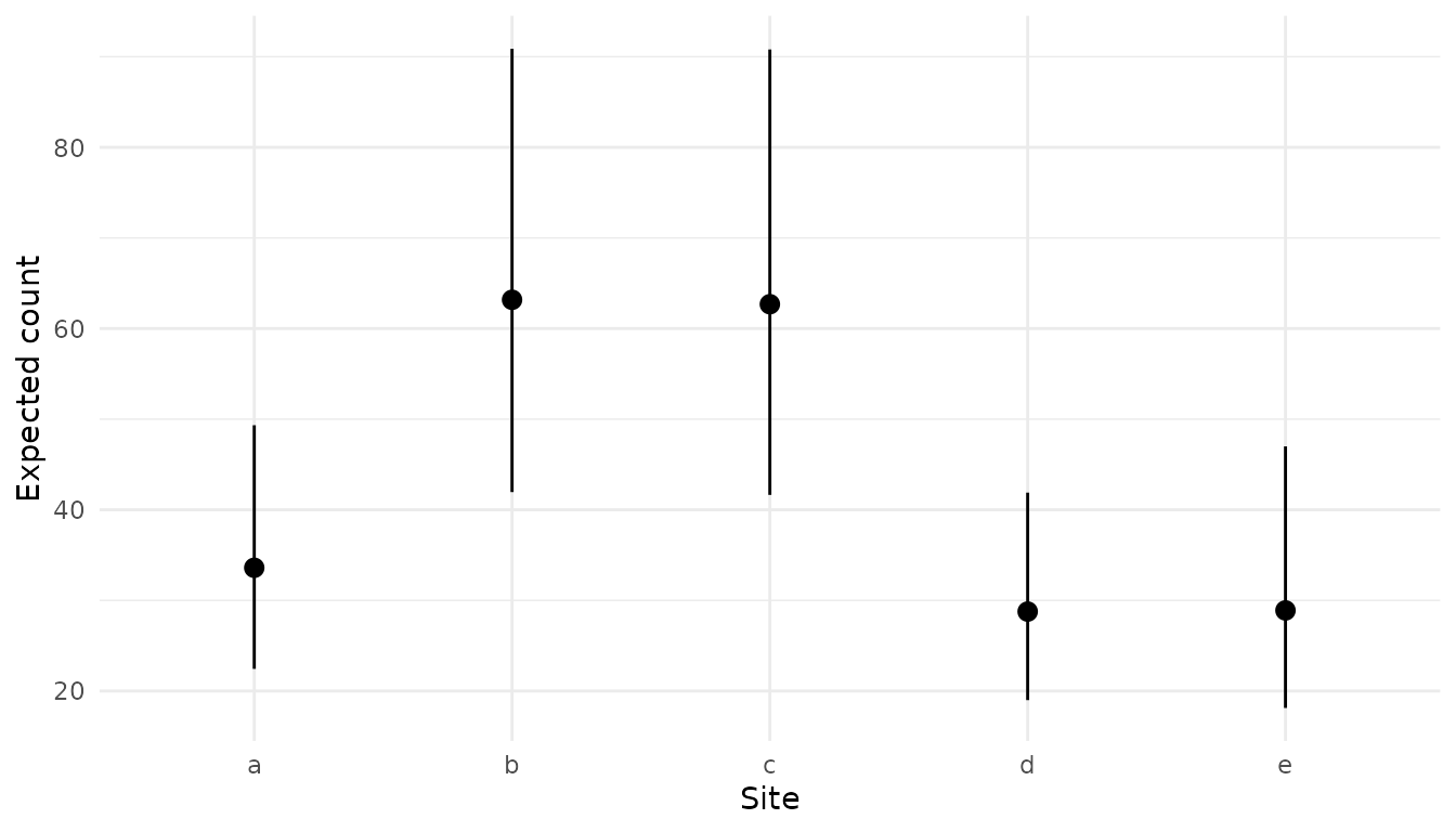

`xobs_only()` for observed combinations only

By default xnew_data(data, site, annual) returns the full 25-row crossed grid:

xnew_data(data, site, annual) |>
  predict(analysis, new_data = _) |>
  nrow()
#> [1] 25

If you only want predictions for the (site, annual) combinations actually observed in the data, wrap them in xobs_only():

xnew_data(data, xobs_only(site, annual)) |>
  predict(analysis, new_data = _) |>
  nrow()
#> [1] 22

22 rows instead of 25: the unbalanced combinations from the design (site e is missing from years 1, 2, and 3).

Casting specific factor levels with `xcast()`

To get specific values of factors, use xcast().

xnew_data(
  data,
  xcast(site = "a", treatment = "restored"),
  temperature = 1
) |>
  predict(analysis, new_data = _)
#> # A tibble: 1 × 9
#>   count site  annual treatment temperature estimate lower upper svalue
#>   <int> <fct> <fct>  <fct>           <dbl>    <dbl> <dbl> <dbl>  <dbl>
#> 1    62 a     1      restored            1     39.0  17.8  89.3   10.6

Note that xnew_data(data, site = "a") will not work: bare = assignment is for continuous covariates (e.g., temperature = 1). To fix a factor at a specific level, wrap it in xcast().

Scalar quantities from `new_expr`

Pass new_data = character(0) to extract a scalar quantity defined in new_expr. term selects which scalar:

predict(analysis, new_data = character(0), term = "eBaseCount")
#> # A tibble: 1 × 9
#>   count site  annual treatment temperature estimate lower upper svalue
#>   <int> <fct> <fct>  <fct>           <dbl>    <dbl> <dbl> <dbl>  <dbl>
#> 1    62 a     1      control          11.9     40.1  19.9  75.3   10.6
predict(analysis, new_data = character(0), term = "eRestoredEffect")
#> # A tibble: 1 × 9
#>   count site  annual treatment temperature estimate lower upper svalue
#>   <int> <fct> <fct>  <fct>           <dbl>    <dbl> <dbl> <dbl>  <dbl>
#> 1    62 a     1      control          11.9     1.73  1.47  2.07   10.6

Random-effect zeroing

By default (random_effects = NULL), a random-effect parameter is zeroed when its associated factor is held at the first level in new_data. This gives the prediction for the ‘typical’ (population-level) group.

Default behaviour

For example, xnew_data(data, temperature) leaves both site and annual at level 1, so both z_bSite and z_bAnnual are zeroed, giving the population-level prediction:

xnew_data(data, temperature) |>
  predict(analysis, new_data = _) |>
  head(3)
#> # A tibble: 3 × 9
#>   count site  annual treatment temperature estimate lower upper svalue
#>   <int> <fct> <fct>  <fct>           <dbl>    <dbl> <dbl> <dbl>  <dbl>
#> 1    62 a     1      control          6.01     29.2  14.6  59.5   10.6
#> 2    62 a     1      control          6.41     29.8  15.0  60.1   10.6
#> 3    62 a     1      control          6.80     30.4  15.4  60.9   10.6

`random_effects = FALSE`

If random_effects = FALSE, zeroing is skipped and predictions use the literal first level of each random-effect factor (here, site = "a" and annual = 1).

xnew_data(data, temperature) |>
  predict(analysis, new_data = _, random_effects = FALSE) |>
  head(3)
#> # A tibble: 3 × 9
#>   count site  annual treatment temperature estimate lower upper svalue
#>   <int> <fct> <fct>  <fct>           <dbl>    <dbl> <dbl> <dbl>  <dbl>
#> 1    62 a     1      control          6.01     32.3  22.2  48.0   10.6
#> 2    62 a     1      control          6.41     32.9  22.9  48.3   10.6
#> 3    62 a     1      control          6.80     33.6  23.7  48.9   10.6

Named list: zero a subset of random effects

Passing a named list overrides the random_effects defined in model(), restricting the set of parameters eligible for zeroing to those listed. Parameters not in the list are kept at their literal value for the first level of their associated factor in new_data. This is useful when you want to marginalize over one random effect while keeping another at a specific level.

xnew_data(data, temperature) |>
  predict(
    analysis,
    new_data = _,
    random_effects = list(z_bSite = "site")
  ) |>
  head(3)
#> # A tibble: 3 × 9
#>   count site  annual treatment temperature estimate lower upper svalue
#>   <int> <fct> <fct>  <fct>           <dbl>    <dbl> <dbl> <dbl>  <dbl>
#> 1    62 a     1      control          6.01     38.9  20.1  71.7   10.6
#> 2    62 a     1      control          6.41     39.7  20.6  72.8   10.6
#> 3    62 a     1      control          6.80     40.6  21.2  73.3   10.6

For the call above (with site and annual both at level 1 in new_data):

z_bSite is listed and site is at level 1, so z_bSite is zeroed (population-mean site, i.e. averaged across sites).
z_bAnnual is not listed, so it is kept at its literal value for annual = 1 — the specific year-1 effect.

This gives the prediction averaged across sites but anchored to year 1 specifically.

Reference data and effect sizes

ref_data must be a flag or a data.frame with one row. When ref_data is a one-row data frame, predict() computes ref_fun2(c(ref_draw, new_draw)) per MCMC iteration, where each element is the scalar posterior draw at the reference row and the new_data row respectively. The returned summary describes the posterior of the transformed quantity, not of the raw prediction. The default ref_fun2 is proportional_change2 from the extras package ((new - ref) / ref), which gives the proportional change of each row in new_data with the ref_data. When ref_data is TRUE, a one-row data.frame is automatically generated with all variables held at reference value.

Proportional change vs control

ref_control <- xnew_data(data, xcast(treatment = "control"))

pred_prop <- xnew_data(data, treatment) |>
  predict(analysis, new_data = _, ref_data = ref_control)

pred_prop
#> # A tibble: 2 × 9
#>   count site  annual treatment temperature estimate lower upper svalue
#>   <int> <fct> <fct>  <fct>           <dbl>    <dbl> <dbl> <dbl>  <dbl>
#> 1    62 a     1      control          11.9    0     0      0       0  
#> 2    62 a     1      restored         11.9    0.734 0.472  1.07   10.6

plot_pointrange(pred_prop, treatment) +
  geom_hline(yintercept = 0, linetype = "dashed") +
  scale_y_continuous(labels = scales::percent) +
  labs(y = "Change vs control", x = "Treatment")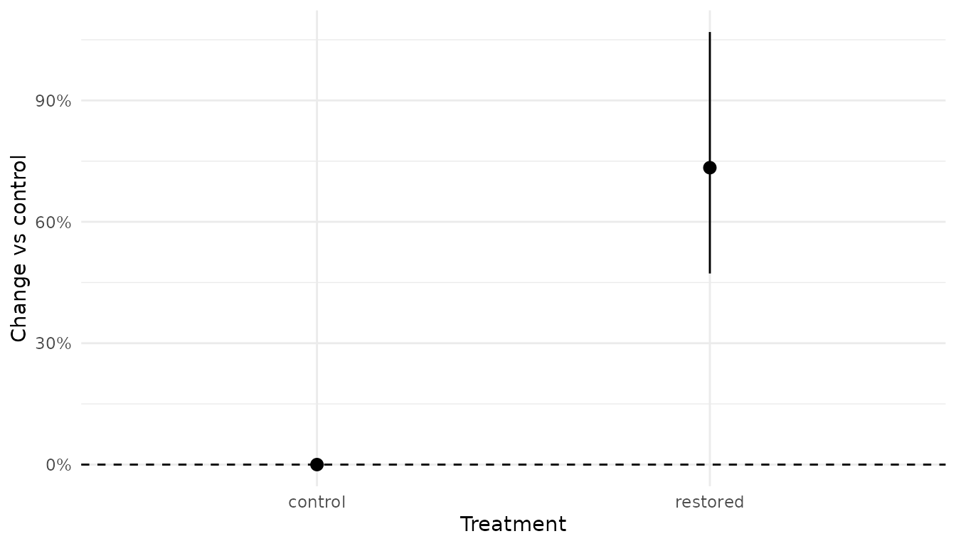

The control row sits at exactly 0%. The restored row gives the proportional change in expected count.

Custom `ref_fun2`: e.g., absolute difference

Pass any function whose first argument takes a vector of two numbers and returns a scalar to summarize a different transformation of the two posteriors. For example, absolute difference reports the effect on the count scale (restored minus control) rather than as a percentage:

pred_diff <- xnew_data(data, treatment) |>
  predict(
    analysis,
    new_data = _,
    ref_data = ref_control,
    ref_fun2 = function(x) x[2] - x[1]
  )

pred_diff
#> # A tibble: 2 × 9
#>   count site  annual treatment temperature estimate lower upper svalue
#>   <int> <fct> <fct>  <fct>           <dbl>    <dbl> <dbl> <dbl>  <dbl>
#> 1    62 a     1      control          11.9      0     0     0      0  
#> 2    62 a     1      restored         11.9     28.9  13.8  58.0   10.6

plot_pointrange(pred_diff, treatment) +
  geom_hline(yintercept = 0, linetype = "dashed") +
  labs(y = "Change vs control (count)", x = "Treatment")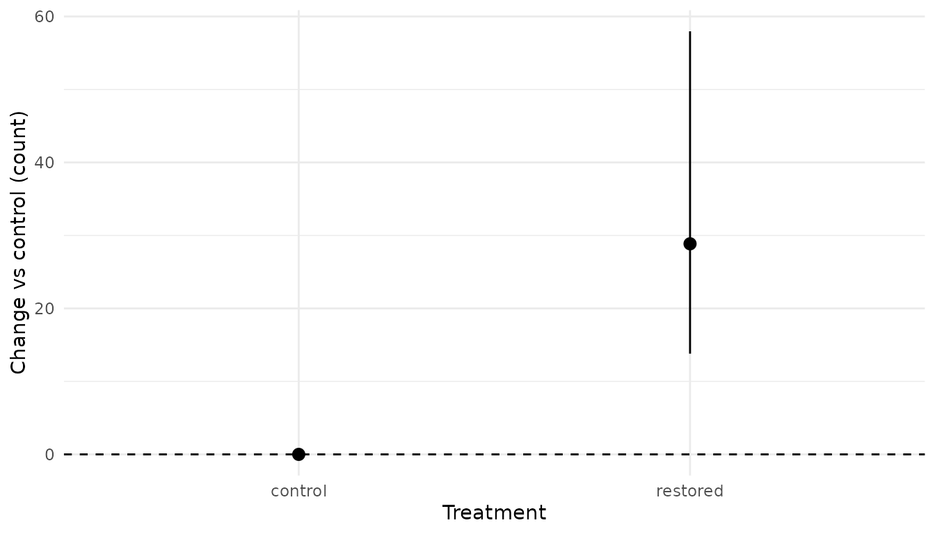

Predicting for an unobserved level

Zeroing a random effect gives the prediction for the typical or average group level, e.g., expected count for an average site, with amongst-site variability removed. However, for a new, unobserved level the uncertainty should be wider to account for amongst-level variation. This is done by drawing a new random effect from its population distribution, which typically will incorporate mean 0 (for random effects centred at 0) and the SD of the random effect, which is estimated. The model’s new_expr already defines an unobserved term to do this:

unobserved[i] <- exp(bIntercept +
  bTreatment[treatment[i]] +
  bTemp * temperature[i] +
  rnorm(1, 0, sSite) +
  rnorm(1, 0, sAnnual))

Setting term = "unobserved" tells predict() to summarize this named quantity from new_expr instead of the default "prediction". Compare the two scopes side-by-side:

typical <- xnew_data(data, treatment) |>
  predict(analysis, new_data = _) |>
  mutate(scope = "typical site")

unobserved <- xnew_data(data, treatment) |>
  predict(analysis, new_data = _, term = "unobserved") |>
  mutate(scope = "unobserved site")

bind_rows(typical, unobserved)
#> # A tibble: 4 × 10
#>   count site  annual treatment temperature estimate lower upper svalue scope    
#>   <int> <fct> <fct>  <fct>           <dbl>    <dbl> <dbl> <dbl>  <dbl> <chr>    
#> 1    62 a     1      control          11.9     40.1 19.9   75.3   10.6 typical …
#> 2    62 a     1      restored         11.9     68.7 34.5  131.    10.6 typical …
#> 3    62 a     1      control          11.9     41.4  9.38 170.    10.6 unobserv…
#> 4    62 a     1      restored         11.9     72.2 15.8  302.    10.6 unobserv…

bind_rows(typical, unobserved) |>
  ggplot(aes(treatment, estimate, ymin = lower, ymax = upper, colour = scope)) +
  geom_pointrange(position = position_dodge(width = 0.3)) +
  theme_minimal() +
  labs(y = "Expected count", x = "Treatment", colour = NULL)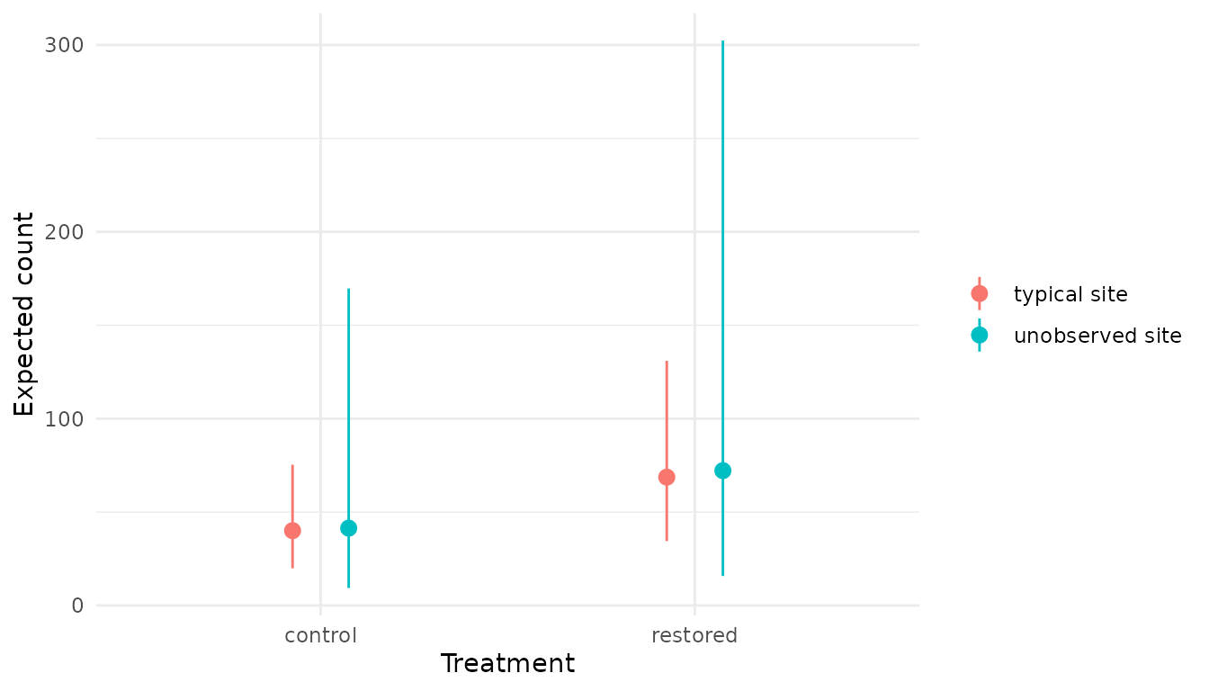

Compatibility limits are wider for unobserved site, as the interval now reflects amongst-site variation in addition to parameter uncertainty.

Overriding `new_expr` and injecting constants

new_expr can be replaced inline as a string. new_values supplies named scalar constants into that expression’s environment. For example, convert counts to biomass by multiplying through a literature or independently measured mean fish mass (g), without refitting the count model:

xnew_data(data, site) |>
  predict(analysis, new_data = _) |>
  head(2)
#> # A tibble: 2 × 9
#>   count site  annual treatment temperature estimate lower upper svalue
#>   <int> <fct> <fct>  <fct>           <dbl>    <dbl> <dbl> <dbl>  <dbl>
#> 1    62 a     1      control          11.9     33.6  22.4  49.3   10.6
#> 2    62 b     1      control          11.9     63.2  42.0  90.9   10.6

predict(
  analysis,
  new_data = xnew_data(data, site),
  new_expr = "
    bSite <- z_bSite * sSite
    for (i in 1:length(site)) {
      prediction[i] <- exp(bIntercept + bSite[site[i]]) * mean_mass_g
    }
  ",
  new_values = list(mean_mass_g = 12)
) |>
  head(2)
#> # A tibble: 2 × 9
#>   count site  annual treatment temperature estimate lower upper svalue
#>   <int> <fct> <fct>  <fct>           <dbl>    <dbl> <dbl> <dbl>  <dbl>
#> 1    62 a     1      control          11.9     403.  269.  592.   10.6
#> 2    62 b     1      control          11.9     758.  503. 1091.   10.6

The second call multiplies the predicted count by an external mean mass of 12 g, giving the posterior of expected biomass per site. Compatibility limits scale proportionally because the constant has no uncertainty attached.

Group-level summaries with `mcmc_derive_data()`

mcmc_derive_data() pairs MCMC samples with the per-row data and returns an mcmc_data object. group_by() + summarize() then aggregates across rows within each group per MCMC iteration to produce per-group posterior distribution summaries.

Total expected count per treatment

mcmc_derive_data(analysis, new_data = data, term = "^eCount$") |>
  group_by(treatment) |>
  summarize() |>
  coef()
#> # A tibble: 2 × 5
#>   treatment estimate lower upper svalue
#>   <fct>        <dbl> <dbl> <dbl>  <dbl>
#> 1 control      3101. 2712. 3569.   10.6
#> 2 restored     5250. 4613. 6059.   10.6

The default summary function is sum, which returns the posterior of total abundance per treatment across all rows.

Custom summary function

Provide any function via .fun. For example, the coefficient of variation of expected count across rows within each treatment:

mcmc_derive_data(analysis, new_data = data, term = "^eCount$") |>
  group_by(treatment) |>
  summarize(.fun = function(x) sd(x) / mean(x)) |>
  coef()
#> # A tibble: 2 × 5
#>   treatment estimate lower upper svalue
#>   <fct>        <dbl> <dbl> <dbl>  <dbl>
#> 1 control      0.461 0.374 0.552   10.6
#> 2 restored     0.492 0.393 0.596   10.6

Combining across analyses with `combine_samples()`

mcmc_data objects come from mcmc_derive_data(); they hold the raw per-row MCMC samples together with the associated data, without the point-estimate-and-limits summarisation that predict() performs.

mcmcr::combine_samples() (with the mcmc_data method from mcmcdata) joins two mcmc_data objects on shared data columns and applies a function to align MCMC draws row-by-row. Its natural use is composing quantities derived from independent analyses: for example, multiplying an abundance posterior by a mass-per-fish posterior to get biomass, where each component was fitted from a different dataset.

Assume a separate mass_analysis was fitted to size-measurement data (different observation model, same site factor), and both analyses expose a per-site quantity:

# Abundance posterior per site, from the counts model fitted above
abundance <- mcmc_derive_data(
  analysis,
  new_data = xnew_data(data, site),
  term = "^eCount$"
)

# Mass-per-fish posterior per site, from a separate analysis (sketch)
mass_per_fish <- mcmc_derive_data(
  mass_analysis,
  new_data = xnew_data(mass_data, site),
  term = "^eMass$"
)

# Per-site biomass posterior: abundance * mass-per-fish
biomass <- mcmcr::combine_samples(
  abundance,
  mass_per_fish,
  by = "site",
  fun = prod
)

by names the data columns to join on (here site); rows present in both inputs are paired. fun is applied to the matched MCMC draws, so prod gives the row-wise product across iterations. The result is an mcmc_data with one row per joined key and a propagated posterior in biomass.

For the two analyses to combine:

MCMC dimensions must match. Both fits need the same number of chains and iterations (e.g. both 3 chains × 500 saved draws). combine_samples() pairs draws position-by-position; mismatched dimensions error out.
by columns must exist in both $data slots. Rows are paired by an inner join, so non-matching rows are dropped silently. Make sure factor levels and column types line up.

Within a single analysis, prefer expressing the composition directly in new_expr; combine_samples() is most useful when the components come from independently fitted models whose draws need joining.

Scalar derived quantities with `mcmc_derive()`

mcmc_derive() returns the raw MCMC samples for one or more scalar terms in new_expr. As with mcmc_derive_data(), this is useful when you want to work with the raw MCMC samples directly rather than predict()’s estimate-and-limits summary.

Unlike predict(), the term argument in mcmc_derive() can accept a regular expression. For example, both eBaseCount and eRestoredEffect are extracted in one call:

scalars <- mcmc_derive(
  analysis,
  new_data = character(0),
  term = "^(eBaseCount|eRestoredEffect)$"
)

coef(scalars)
#> # A tibble: 2 × 5
#>   term            estimate lower upper svalue
#>   <term>             <dbl> <dbl> <dbl>  <dbl>
#> 1 eBaseCount         40.1  19.9  75.3    10.6
#> 2 eRestoredEffect     1.73  1.47  2.07   10.6

coef() is run on the mcmc_derive() output to get point estimates with compatibility limits.

Arithmetic on `mcmcr` objects

Quantities you anticipate are usually cleanest to define directly in new_expr and pull with predict(). Raw mcmcr arithmetic earns its keep when the question requires composing outputs of different post-fit operations — for example, combining a group-aggregated quantity from mcmc_derive_data() with a scalar from mcmc_derive(), or producing summaries predict() cannot (probability statements, custom posterior quantiles).

First, get totals per treatment, then extract each row as raw MCMC draws:

totals <- mcmc_derive_data(analysis, new_data = data, term = "^eCount$") |>
  group_by(treatment) |>
  summarize()

restored_total <- as.mcmcr(filter(totals, treatment == "restored"))[[1]]
control_total <- as.mcmcr(filter(totals, treatment == "control"))[[1]]

The posterior of the absolute difference in total expected catch (restored minus control), summed over the observed design — a count-scale effect size that eRestoredEffect (a multiplicative ratio) doesn’t quantify:

extra_catch <- restored_total - control_total
coef(extra_catch)
#> # A tibble: 1 × 5
#>   term      estimate lower upper svalue
#>   <term>       <dbl> <dbl> <dbl>  <dbl>
#> 1 parameter    2147. 1450. 3010.   10.6

And the posterior probability that restoration adds at least 2000 fish in total — a question predict() cannot answer:

mean(extra_catch >= 2000)
#> [1] 0.6606667

Cheat sheet

Goal	Tool
Posterior summary at new covariate values	`predict()`
Posterior summary for a scalar derived quantity	`predict()` with `new_data = character(0)` and `term` specified
Prediction for an unobserved factor level (includes amongst-level variation)	`new_expr` term with `rnorm(1, 0, s*)` for the random effect
Effect size (proportional, absolute)	`predict()` with `ref_data` + `ref_fun2`
Group-level aggregates (sum, mean, custom) per MCMC iteration	`mcmc_derive_data()` + `group_by()` + `summarize()`
Combine quantities derived from independent analyses	`mcmcr::combine_samples()`
Scalar parameter posteriors and arithmetic	`mcmc_derive()`

See ?predict.mb_analysis, ?mcmc_derive.mb_analysis, ?mcmc_derive_data.mb_analysis, and ?mcmcr::combine_samples for full argument documentation.

Setup: fit demo model

Default prediction

Covariate grids with the newdata helpers

Continuous covariate

Specific values via xnew_seq() or with =

Single factor

xobs_only() for observed combinations only

Casting specific factor levels with xcast()

Scalar quantities from new_expr