Beta-binomial Deviance Residuals • extras

Beta-binomial distribution

The beta-binomial distribution is useful when we wish to incorporate additional variation into the probability parameter of the binomial distribution, p. It accomplishes this by drawing p from a beta distribution. The parameters of the beta-binomial are the number of trials, n, and the shape parameters of the beta distribution, \alpha and \beta.

The likelihood of the beta-binomial can be described as follows: P(x | n, \alpha, \beta) = \frac{\Gamma(n + 1)}{\Gamma(x + 1)\Gamma(n - x + 1)} \frac{\Gamma(x + \alpha) \Gamma(n - x + \beta)}{\Gamma(n + \alpha + \beta)} \frac{\Gamma(\alpha + \beta)}{\Gamma(\alpha) \Gamma(\beta)}, where x is a natural number ≤ n, \alpha and \beta are >0, and where \Gamma() represents the gamma function.

The log-likelihood is:
\log(P(x | n, \alpha, \beta)) = \log(\Gamma(n + 1)) - \log(\Gamma(x + 1)) - \log(\Gamma(n - x + 1)) + \log(\Gamma(x + \alpha)) + \\ \log(\Gamma(n - x + \beta)) - \log(\Gamma(n + \alpha + \beta)) + \log(\Gamma(\alpha + \beta)) - \log(\Gamma(\alpha)) - \log(\Gamma(\beta)).

The expected value of the beta-binomial distribution is n \cdot \frac{\alpha}{\alpha + \beta}. This is the same as the expected value of the binomial distribution (n \cdot p), with the p replaced by the expected value of the beta distribution, \frac{\alpha}{\alpha + \beta}.

A parameterization frequently used for the beta-binomial distribution uses this expected probability (p) as a parameter, with a dispersion parameter (\theta) that specifies the variance in the probability. Our particular parameterization of \theta is slightly unconventional, but has useful properties when modelling. When \theta = 0, the beta-binomial reverts to the binomial distribution. When \theta = 1 and p = 0.5, the parameters of the beta distribution become \alpha = 1 and \beta = 1, which correspond to a uniform distribution for the beta-binomial probability parameter.

The relationships between p and \theta and \alpha and \beta are defined as follows:
p = \frac{\alpha}{\alpha + \beta} \theta = \frac{2}{\alpha + \beta}

\alpha = 2\cdot\frac{p}{\theta} \beta = 2\cdot\frac{1 - p}{\theta}

Deviance:

Recall that the likelihood of a model is the probability of the data set given the model (P(\text{data}|\text{model})). The deviance of a model, D, is defined by: D(\text{model},\text{data}) = 2(\log(P(\text{data}|\text{saturated model})) - \log(P(\text{data}|\text{fitted model}))), where the saturated model is the model that perfectly fits the data.

The saturated model usually uses the value of x in place of the mean parameter, thereby fitting through the data points. For example, calculating the saturated log-likelihood of the normal distribution involves using the x value(s) in place of the mean parameter \mu in the log-likelihood. Recall from above that the expected value of the binomial distribution is n \cdot p. Since n is fixed in the binomial distribution, p = \frac{x}{n} is used to calculate the saturated log-likelihood.

In the case of the beta-binomial distribution, there is some confusion about what should be used as the saturated model. One suggested approach is to use the saturated log-likelihood of the binomial distribution, as described above, effectively setting the \theta dispersion term to 0. A second suggested approach is to use the same method as described for the binomial distribution (i.e., replacing p with \frac{x}{n}), and holding the \theta value constant. Both of these approaches have issues.

The problem with the first approach is that likelihood profile of the beta-binomial becomes increasingly dispersed relative to the binomial as \theta increases (Fig. 1). Consequently, increasing \theta increases the deviance even if the expected value of the fitted model is the same as the saturated binomial model.

$Fig. 1: Beta-binomial likelihood profile for $x = 1$ and $n = 5$, for different values of $\theta$. $\theta = 0$ corresponds to the binomial case.$

Fig. 1: Beta-binomial likelihood profile for x = 1 and n = 5, for different values of \theta. \theta = 0 corresponds to the binomial case.

The problem with the second approach is that for some combinations of p and \theta, the resultant deviance values are negative. This is an issue for two reasons. Firstly, it is nonsensical because by definition the saturated model should be the best possible fit to the data. Secondly, it is computationally problematic, because calculating deviance residuals, as we will do in the next section, involves taking the square root of the deviance.

Here is an example of a case where the deviance is negative. Using x = 1, n = 5, p = 0.3, and \theta = 0.5, we calculate the saturated log-likelihood:

\alpha_{sat} = \frac{2 (\frac{x}{n})}{\theta} = \frac{2(0.3)}{0.5} = 0.8 \beta_{sat} = \frac{2 (1 - \frac{x}{n})}{\theta} = \frac{2 (1 - 0.3)}{0.5} = 3.2

\log(P(x|n, p_{sat}, \theta_{sat}) = -1.355106,

the fitted log-likelihood:

\alpha_{fit} = \frac{2 (p)}{\theta} = \frac{2(0.3)}{0.5} = 1.2 \beta_{fit} = \frac{2 (1 - p)}{\theta} = \frac{2 (1 - 0.3}{0.5} = 2.8

\log(P(x|n, p_{fit}, \theta_{fit})) = -1.32999,

and finally, the deviance:

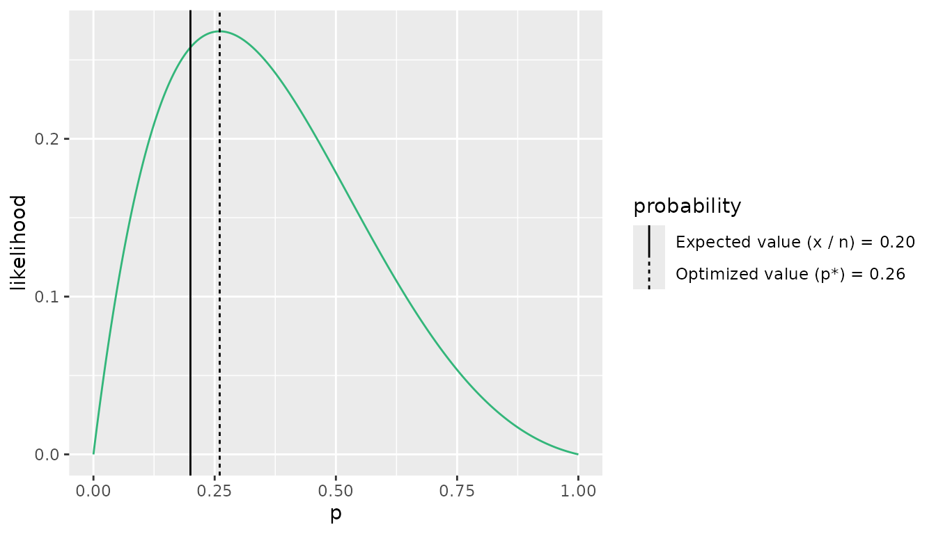
\begin{aligned} D(n, p, \theta, x) &= 2(\log(P(x|n, p_{sat}, \theta_{sat})) - \log(P(x|n, p_{fit}, \theta_{fit}))) \\ &= 2(-1.355106 - -1.32999) \\ &= -0.050232. \end{aligned}

In summary, the deviance is negative because the likelihood at the expected value, p = \frac{x}{n} is less than the likelihood of the observed value (Fig. 2).

The solution to the problem appears to be to choose the value of p that maximizes the likelihood. However, the beta-binomial distribution has closed-form solutions only for certain values of \alpha and \beta. Thus, we must generally search for the value of p that maximizes the likelihood for each data point in order to calculate the saturated log-likelihood. We will refer to the optimized p value for the i^{th} data point as p_i^*, and generally as p^*. We use p^* to calculate the saturated log-likelihood that produces deviances that are (a) strictly positive, and (b) relative to the value of \theta. The value of p_i^* for the example case with x = 1, n = 5, and \theta = 0.5 is shown in Figure 2.

$Fig. 2: Beta-binomial likelihood profile for $x = 1$, $n = 5$, and $\theta = 0.5$. The dashed vertical line shows the likelihood at the expected value of the beta-binomial distribution ($n \cdot p$) where $p = \frac{x}{n} = \frac{1}{5} = 0.2$. As you can see, this is not the $p$ for which the likelihood is maximized. The solid vertical line shows the likelihood at its maximum point. In this case, $p^* = 0.26$.$

Fig. 2: Beta-binomial likelihood profile for x = 1, n = 5, and \theta = 0.5. The dashed vertical line shows the likelihood at the expected value of the beta-binomial distribution (n \cdot p) where p = \frac{x}{n} = \frac{1}{5} = 0.2. As you can see, this is not the p for which the likelihood is maximized. The solid vertical line shows the likelihood at its maximum point. In this case, p^* = 0.26.

Deviance residuals

The unit deviance, d_i refers to the deviance for the i^{th} data point, x_i:
d_i = 2(\log(P(x_i|n, p_i^*, \theta)) - \log(P(x_i|n, p, \theta))). The deviance residual is the signed squared root of the unit deviance,
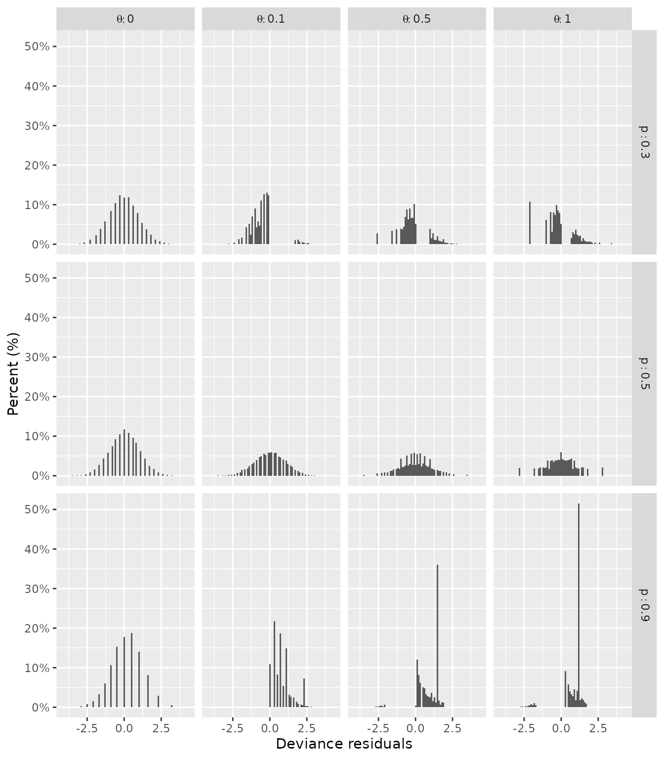
r_i = \text{sign}(x_i - (n p_i^*)) \sqrt{d_i}. The following plot shows histograms of deviance residuals for 10,000 randomly generated data points with n = 50 and various values of p and \theta.

$Fig. 4: Histograms of deviance residuals for 10,000 beta-binomial data points simulated with $n = 50$, $p = \{0.3, 0.5, 0.9 \}$, and $\theta = \{0.0, 0.1, 0.5, 1.0 \}$. The percentages within each panel (i.e., each combination of $p$ and $\theta$) sum to 100%.$

Fig. 4: Histograms of deviance residuals for 10,000 beta-binomial data points simulated with n = 50, p = \{0.3, 0.5, 0.9 \}, and \theta = \{0.0, 0.1, 0.5, 1.0 \}. The percentages within each panel (i.e., each combination of p and \theta) sum to 100%.

Recall that \theta = 0 refers to the binomial case. When p = 0.5 and \theta > 0, deviance residuals close to 0 become less common; as \theta increases, the distribution of deviance residuals becomes less continuous (Fig. 4). When p deviates from 0.5 and \theta > 0, the distribution of the deviance residuals becomes increasingly skewed and discontinuous (Fig. 4).

Due to the skewed and discontinuous nature of the distribution of the deviance residuals, the goodness of fit of a beta-binomial model cannot be assessed from the deviance residuals alone but must be evaluated using posterior predictive checking.